25. matplotlib.pyplot 2부#
참고
웨스 맥키니의 <파이썬 라이브러리를 활용한 데이터 분석>의 9장1절에 사용된 소스코드의 일부를 활용한다.
기본 설정
import numpy as np
import pandas as pd
맷플롯립Matplotlib은 간단한 그래프 도구를 제공하는 라이브러리다.
맷플롯립의 대부분의 함수는 파이플롯pyplot 모듈에 포함되어 있으며
관행적으로 plt 별칭으로 불러온다.
import matplotlib.pyplot as plt
datetime.datetime 자료형은 시간(날짜) 데이터를 다룬다.
from datetime import datetime
25.1. Figure 객체와 서브플롯(subplot)#
모든 그래프는 Figure 객체 내에 존재하며, plt.figure() 함수에 의해 생성된다.
fig = plt.figure()
Figure 객체 내에 그래프를 그리려면 서브플롯(subplot)을 지정해야 한다.
아래 코드는 add_subplot() 함수를 이용하여 지정된 Figure 객체안에 그래프를 그릴 공간을 준비한다.
(nrows, ncols, index) 형식의 인자의 의미는 다음과 같다.
nrows: 이미지 행의 개수
ncols: 이미지 칸의 개수
index: 이미지의 인덱스. 1부터 시작.
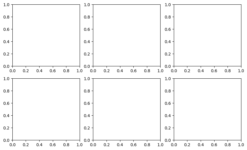
만약 2x2 모양으로 총 4개의 이미지를 생성하려면 아래와 같이 실행한다.
fig = plt.figure()

ax1 = fig.add_subplot(2, 2, 1)
ax2 = fig.add_subplot(2, 2, 2)
ax3 = fig.add_subplot(2, 2, 3)
ax4 = fig.add_subplot(2, 2, 4)
그래프 삽입하기
두 가지 방식으로 각각의 서브플롯에 그림을 삽입할 수 있다.
방식 1: matplotlib.pyplot.plot() 함수 활용
이 방식은 항상 마지막에 선언된 서브플롯에 그래프를 그린다. 예를 들어 아래 코드는 무작위로 선택된 50개의 정수들의 누적합으로 이루어진 데이터를 파선 그래프로 그린다.
np.random.seed(12345)

data1 = np.random.randn(50).cumsum()
data2 = np.random.randn(50).cumsum()
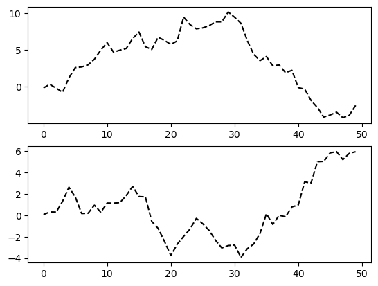
2x1 모양의 2개 이미지 사용하기
fig = plt.figure()

ax1 = fig.add_subplot(2, 1, 1)
plt.plot(data1, 'k--')

ax2 = fig.add_subplot(2, 1, 2)
plt.plot(data2, 'k--')
[<matplotlib.lines.Line2D at 0x1bd35648220>]
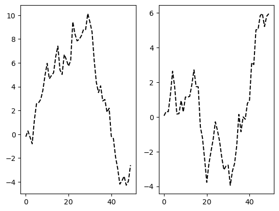
1x2 모양의 2개 이미지 사용하기
fig = plt.figure()

ax1 = fig.add_subplot(1, 2, 1)
plt.plot(data1, 'k--')

ax2 = fig.add_subplot(1, 2, 2)
plt.plot(data2, 'k--')
[<matplotlib.lines.Line2D at 0x1bd35786ad0>]
방식 2: 객체명.plot() 함수 활용
특정 서브플롯에 그래프를 삽입하려면 서브플롯 객체의 이름과 함께 plot() 함수 등을 호출해야 한다.
np.random.seed(12345)

fig = plt.figure()
ax1 = fig.add_subplot(2, 2, 1)
ax2 = fig.add_subplot(2, 2, 2)
ax3 = fig.add_subplot(2, 2, 3)
ax4 = fig.add_subplot(2, 2, 4)

# 위치: (2, 2, 1)
ax1.hist(np.random.randn(100), bins=20, color='k', alpha=.1)
# 위치: (2, 2, 2)
ax2.scatter(np.arange(30), np.arange(30) + 3 * np.random.randn(30))
# 위치: (2, 2, 3)
ax3.plot(np.random.randn(50).cumsum(), 'k--')
# 위치: (2, 2, 4)
ax4.plot(np.random.randn(50).cumsum(), 'k--')

plt.show()
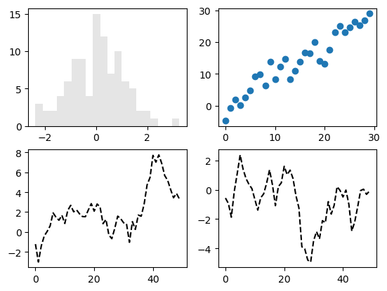
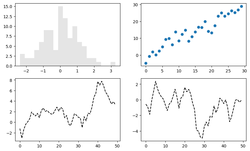
Figure 객체의 크기는 plt.rc() 함수를 이용해서 아래와 같이 지정한다.
plt.rc() 함수의 자세한 활용법은 잠시 뒤에 보다 자세히 살펴 본다.
plt.rc('figure', figsize=(10, 6))
이제 네 개의 이미지가 보다 적절한 크기로 그려진다.
np.random.seed(12345)

fig = plt.figure()
ax1 = fig.add_subplot(2, 2, 1)
ax2 = fig.add_subplot(2, 2, 2)
ax3 = fig.add_subplot(2, 2, 3)
ax4 = fig.add_subplot(2, 2, 4)

# 위치: (2, 2, 1)
ax1.hist(np.random.randn(100), bins=20, color='k', alpha=.1)
# 위치: (2, 2, 2)
ax2.scatter(np.arange(30), np.arange(30) + 3 * np.random.randn(30))
# 위치: (2, 2, 3)
ax3.plot(np.random.randn(50).cumsum(), 'k--')
# 위치: (2, 2, 4)
ax4.plot(np.random.randn(50).cumsum(), 'k--')

plt.show()
서브플롯 관리
matplotlib.pyplot.subplots() 함수는 여러 개의 서브플롯을 포함하는 Figure 객체를 관리해준다.
예를 들어, 아래 코드는 2x3 크기의 서브플롯을 담은 (2,3) 모양의 넘파이 어레이로 생성한다.
반환값:
Figure객체와 지정된 크기의 넘파이 어레이. 각 항목은 서브플롯 객체임.
fig, axes = plt.subplots(2, 3)
axes
array([[<Axes: >, <Axes: >, <Axes: >],
       [<Axes: >, <Axes: >, <Axes: >]], dtype=object)
x 축 또는 y 축 눈금을 공유할 수 있다.
fig, axes = plt.subplots(2, 3, sharex=True, sharey=True)
axes
array([[<Axes: >, <Axes: >, <Axes: >],
       [<Axes: >, <Axes: >, <Axes: >]], dtype=object)
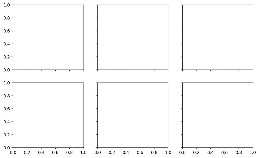
plt.subplots_adjust() 함수는 각 서브플롯 사이의 여백을 조절하는 방식을 보여준다.
여백의 크기는 그래프의 크기와 숫자에 의존한다.
여백이 0일 때:
fig, axes = plt.subplots(2, 2, sharex=True, sharey=True)

for i in range(2):
    for j in range(2):
        axes[i, j].plot(np.random.randn(50))

plt.subplots_adjust(wspace=0, hspace=0) # 상하좌우 여백: 0
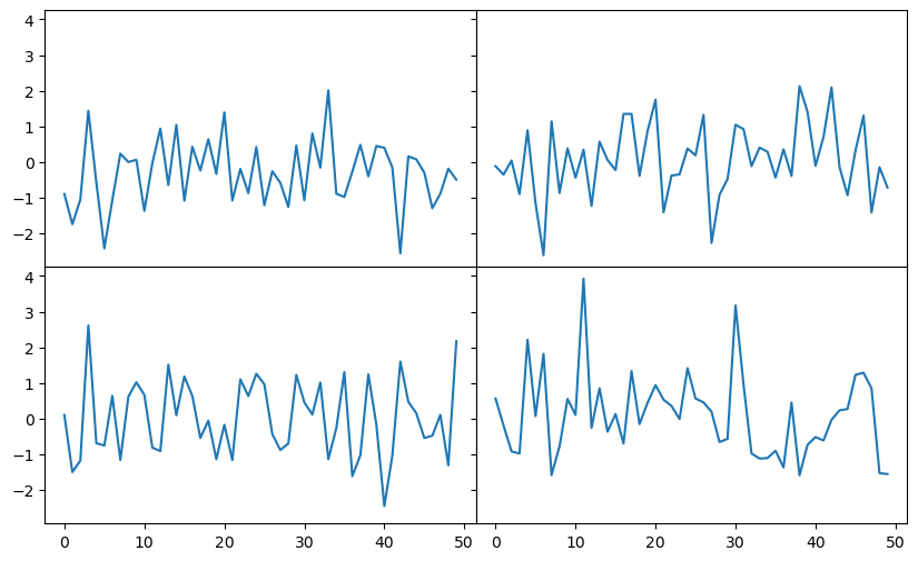
여백이 0.1일 때:
fig, axes = plt.subplots(2, 2, sharex=True, sharey=True)

for i in range(2):
    for j in range(2):
        axes[i, j].plot(np.random.randn(50))

plt.subplots_adjust(wspace=0.1, hspace=0.1) # 상하좌우 여백: 0.1
25.2. 눈금과 라벨#
이미지 타이틀, 축 이름, 눈금, 눈금 이름 지정
두 가지 방식으로 진행할 수 있다.
방식 1: 파이플롯 객체의 메서드 활용
set_xticks()함수: 눈금 지정set_xticklabels()함수: 눈금 라벨 지정set_title()함수: 그래프 타이틀 지정set_xlabel()함수: x축 이름 지정
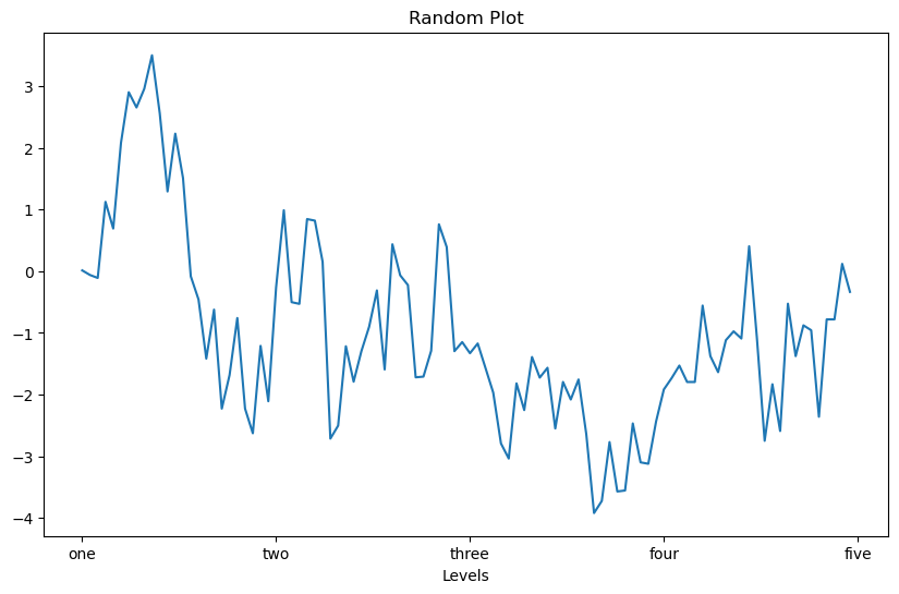
data = np.random.randn(100).cumsum()
fig = plt.figure()
ax = fig.add_subplot(1, 1, 1)
ax.plot(data)

ticks = ax.set_xticks([0, 25, 50, 75, 100])
labels = ax.set_xticklabels(['one', 'two', 'three', 'four', 'five'])

ax.set_title('Random Plot')
ax.set_xlabel('Levels')
Text(0.5, 0, 'Levels')
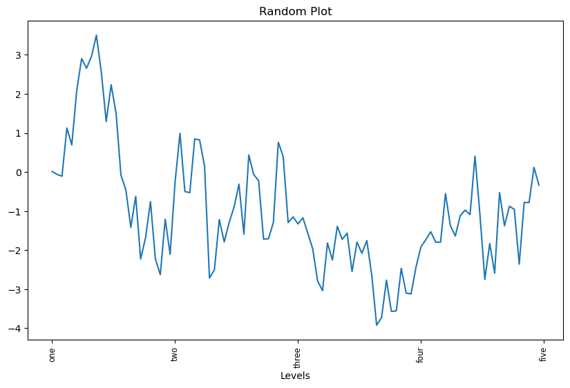
눈금 크기와 방향도 지정할 수 있다.
fig = plt.figure()
ax = fig.add_subplot(1, 1, 1)
ax.plot(data)

ticks = ax.set_xticks([0, 25, 50, 75, 100])
labels = ax.set_xticklabels(['one', 'two', 'three', 'four', 'five'],
                            rotation=90, fontsize='small')

ax.set_title('Random Plot')
ax.set_xlabel('Levels')
Text(0.5, 0, 'Levels')
방식 2: pyplot 모듈의 함수 활용
이 방식은 마지막에 선언된 서브플롯에 대해서만 작동한다.
plt.xticks()함수: 눈금 및 눈금 라벨 지정plt.title()함수: 그래프 타이틀 지정plt.xlabel()함수: x축 이름 지정
fig = plt.figure()
ax = fig.add_subplot(1, 1, 1)
ax.plot(data)

plt.xticks([0, 25, 50, 75, 100], ['one', 'two', 'three', 'four', 'five'],
            rotation=90, fontsize='small')

plt.title('Random Plot')
plt.xlabel('Levels')
Text(0.5, 0, 'Levels')
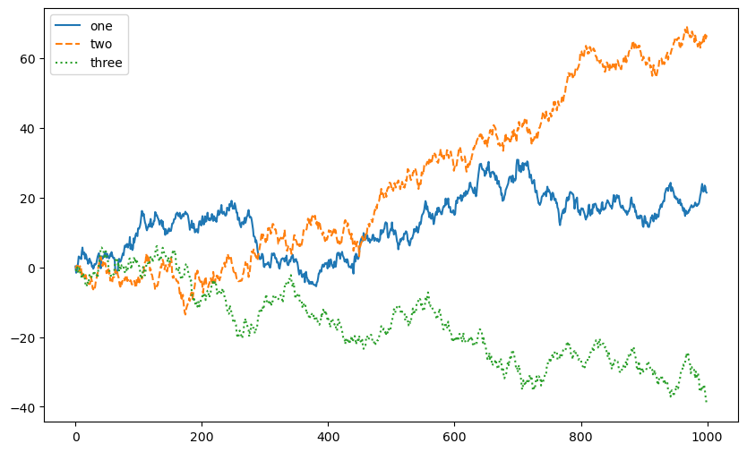
np.random.seed(17)

fig, ax = plt.subplots()
ax.plot(np.random.randn(1000).cumsum(), label="one")
ax.plot(np.random.randn(1000).cumsum(), linestyle="dashed", label="two")
ax.plot(np.random.randn(1000).cumsum(), linestyle="dotted", label="three")
ax.legend()
<matplotlib.legend.Legend at 0x1bd37f0a4a0>
25.3. 그래프 저장#
가장 최근에 생성된 그래프를 가리키는 Figure 객체를 이미지 파일로 저장할 수 있다.
fig
type(fig)
matplotlib.figure.Figure
Figure 객체의 savefig() 함수를 이용한다.
파일명의 확장장에 맞춰 적절한 포맷format으로 저장되며,
dpi를 지정하여 저장된 이미지 파일의 해상도를 조절할 수 있다.
fig.savefig("./images/random.png", dpi=400)
dpi
dpi는 dots for inch, 즉 1인치(2.54cm)당 디지털 프린터가 찍을 수 있는 점(dot)의 수를 가리키며, 값이 클 수록 저장된 사진의 해상도가 높아진다.
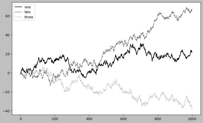
25.4. 그래프 스타일 지정#
plt.style.use('grayscale')
np.random.seed(17)

fig, ax = plt.subplots()
ax.plot(np.random.randn(1000).cumsum(), label="one")
ax.plot(np.random.randn(1000).cumsum(), linestyle="dashed", label="two")
ax.plot(np.random.randn(1000).cumsum(), linestyle="dotted", label="three")
ax.legend()
<matplotlib.legend.Legend at 0x1bd37f659f0>
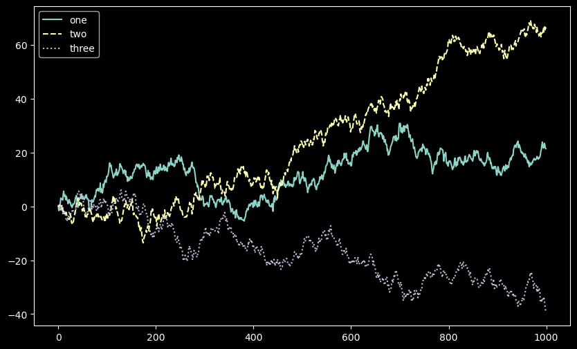
plt.style.use('dark_background')
np.random.seed(17)

fig, ax = plt.subplots()
ax.plot(np.random.randn(1000).cumsum(), label="one")
ax.plot(np.random.randn(1000).cumsum(), linestyle="dashed", label="two")
ax.plot(np.random.randn(1000).cumsum(), linestyle="dotted", label="three")
ax.legend()
<matplotlib.legend.Legend at 0x1bd37fefa90>
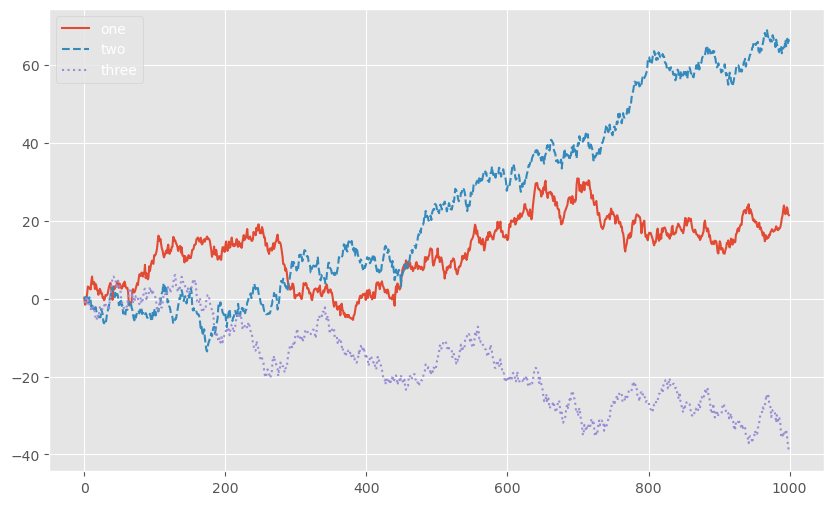
plt.style.use('ggplot')
np.random.seed(17)

fig, ax = plt.subplots()
ax.plot(np.random.randn(1000).cumsum(), label="one")
ax.plot(np.random.randn(1000).cumsum(), linestyle="dashed", label="two")
ax.plot(np.random.randn(1000).cumsum(), linestyle="dotted", label="three")
ax.legend()
<matplotlib.legend.Legend at 0x1bd37f65930>
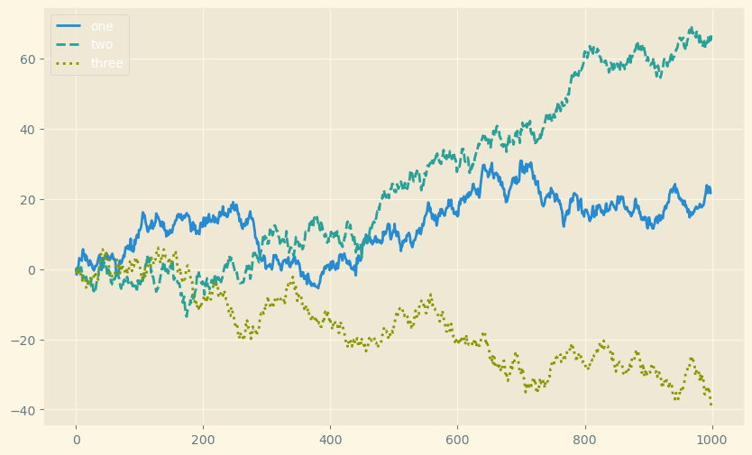
plt.style.use('Solarize_Light2')
np.random.seed(17)

fig, ax = plt.subplots()
ax.plot(np.random.randn(1000).cumsum(), label="one")
ax.plot(np.random.randn(1000).cumsum(), linestyle="dashed", label="two")
ax.plot(np.random.randn(1000).cumsum(), linestyle="dotted", label="three")
ax.legend()
<matplotlib.legend.Legend at 0x1bd321d0820>
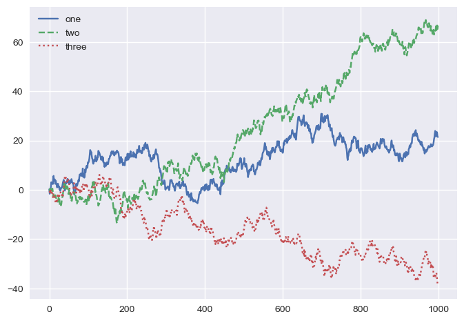
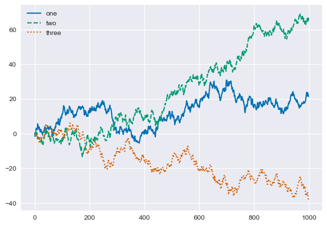
plt.style.use('seaborn-v0_8')
np.random.seed(17)

fig, ax = plt.subplots()
ax.plot(np.random.randn(1000).cumsum(), label="one")
ax.plot(np.random.randn(1000).cumsum(), linestyle="dashed", label="two")
ax.plot(np.random.randn(1000).cumsum(), linestyle="dotted", label="three")
ax.legend()
<matplotlib.legend.Legend at 0x1bd377798a0>
plt.style.use('seaborn-v0_8-colorblind')
np.random.seed(17)

fig, ax = plt.subplots()
ax.plot(np.random.randn(1000).cumsum(), label="one")
ax.plot(np.random.randn(1000).cumsum(), linestyle="dashed", label="two")
ax.plot(np.random.randn(1000).cumsum(), linestyle="dotted", label="three")
ax.legend()
<matplotlib.legend.Legend at 0x1bd38cdf9d0>
25.5. matplotlib 기본 설정#
plt.rc() 함수를 이용하여 matplot을 이용하여 생성되는 이미지 관련 설정을 전역적으로 지정할 수 있다.
사용되는 형식은 다음과 같다.
첫째 인자: 속성 지정
둘째 인자: 속성값 지정
참고: ‘rc’ 는 기본설정을 의미하는 단어로 많이 사용된다. 풀어 쓰면 “Run at startup and they Configure your stuff”, 즉, “프로그램이 시작할 때 기본값들을 설정한다”의 의미이다. ‘.vimrc’, ‘.bashrc’, ‘.zshrc’ 등 많은 애플리케이션의 초기설정 파일명에 사용되곤 한다.
아래 코드는 다양한 속성을 지정하는 방식을 보여준다.
이미지 사이즈 지정
plt.rc('figure', figsize=(10, 6))
선 속성 지정
plt.rc('lines', linewidth=3, color='b')
텍스트 폰트 속성 지정
font_options = {'family' : 'serif',
                'weight' : 'bold',
                'size'   : '13'}

plt.rc('font', **font_options) # plt.rc('font', family='serif', weight='bold', size=13)
그래프 구성 요소의 색상 지정
plt.rcParams['text.color'] = 'red'
plt.rcParams['xtick.color'] = 'green'
plt.rcParams['ytick.color'] = '#CD5C5C'  # RGB 색상
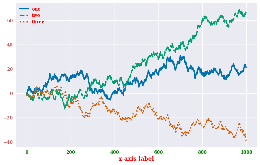
아래 코드는 앞서 설정된 다양한 속성을 반영한 결과를 보여준다.
np.random.seed(17)

fig, ax = plt.subplots()
ax.plot(np.random.randn(1000).cumsum(), label="one")
ax.plot(np.random.randn(1000).cumsum(), linestyle="dashed", label="two")
ax.plot(np.random.randn(1000).cumsum(), linestyle="dotted", label="three")

ax.set_xlabel("x-axis label")
ax.legend()
<matplotlib.legend.Legend at 0x1bd38d5e6b0>
plt.close('all')