시계열 데이터

28. 시계열 데이터#

import numpy as np
import pandas as pd

PREVIOUS_MAX_ROWS = pd.options.display.max_rows
pd.options.display.max_columns = 20
pd.options.display.max_rows = 20
pd.options.display.max_colwidth = 80

np.random.seed(12345)
np.set_printoptions(precision=4, suppress=True)

import matplotlib.pyplot as plt

plt.rc("figure", figsize=(10, 6))

28.1. `datetime` 자료형#

from datetime import datetime

now = datetime.now()
now

datetime.datetime(2023, 5, 26, 1, 21, 40, 533281)

print(now.year, now.month, now.day)

2023 5 26

delta = datetime(2011, 1, 7) - datetime(2009, 6, 24, 8, 15)
delta

datetime.timedelta(days=561, seconds=56700)

delta.days

delta.seconds

from datetime import timedelta

start = datetime(2011, 1, 7)

start + timedelta(12)

datetime.datetime(2011, 1, 19, 0, 0)

start - 2 * timedelta(12)

datetime.datetime(2010, 12, 14, 0, 0)

28.1.1. 문자열과 `Datetime`#

stamp = datetime(2011, 1, 3)

str(stamp)

'2011-01-03 00:00:00'

stamp.strftime("%Y-%m-%d")

'2011-01-03'

value = "2011-01-03"
datetime.strptime(value, "%Y-%m-%d")

datetime.datetime(2011, 1, 3, 0, 0)

datestrs = ["7/6/2011", "8/6/2011"]
[datetime.strptime(x, "%m/%d/%Y") for x in datestrs]

[datetime.datetime(2011, 7, 6, 0, 0), datetime.datetime(2011, 8, 6, 0, 0)]

pd.to_datetime() 함수

datestrs = ["2011-07-06 12:00:00", "2011-08-06 00:00:00"]
pd.to_datetime(datestrs)

DatetimeIndex(['2011-07-06 12:00:00', '2011-08-06 00:00:00'], dtype='datetime64[ns]', freq=None)

idx = pd.to_datetime(datestrs + [None])
idx

DatetimeIndex(['2011-07-06 12:00:00', '2011-08-06 00:00:00', 'NaT'], dtype='datetime64[ns]', freq=None)

idx[2]

NaT

pd.isna(idx)

array([False, False,  True])

28.2. 시계열 데이터 기초#

dates = [datetime(2011, 1, 2), datetime(2011, 1, 5),
         datetime(2011, 1, 7), datetime(2011, 1, 8),
         datetime(2011, 1, 10), datetime(2011, 1, 12)]

ts = pd.Series(np.random.standard_normal(6), index=dates)
ts

2011-01-02   -0.204708
2011-01-05    0.478943
2011-01-07   -0.519439
2011-01-08   -0.555730
2011-01-10    1.965781
2011-01-12    1.393406
dtype: float64

ts.index

DatetimeIndex(['2011-01-02', '2011-01-05', '2011-01-07', '2011-01-08',
               '2011-01-10', '2011-01-12'],
              dtype='datetime64[ns]', freq=None)

ts + ts[::2]

2011-01-02   -0.409415
2011-01-05         NaN
2011-01-07   -1.038877
2011-01-08         NaN
2011-01-10    3.931561
2011-01-12         NaN
dtype: float64

ts.index

DatetimeIndex(['2011-01-02', '2011-01-05', '2011-01-07', '2011-01-08',
               '2011-01-10', '2011-01-12'],
              dtype='datetime64[ns]', freq=None)

ts.index.dtype

dtype('<M8[ns]')

stamp = ts.index[0]
stamp

Timestamp('2011-01-02 00:00:00')

28.2.1. 인덱싱, 선택, 슬라이싱#

stamp = ts.index[2]
ts[stamp]

-0.5194387150567381

ts["2011-01-10"]

1.9657805725027142

longer_ts = pd.Series(np.random.standard_normal(1000),
                      index=pd.date_range("2000-01-01", periods=1000))
longer_ts

2000-01-01    0.092908
2000-01-02    0.281746
2000-01-03    0.769023
2000-01-04    1.246435
2000-01-05    1.007189
                ...   
2002-09-22    0.930944
2002-09-23   -0.811676
2002-09-24   -1.830156
2002-09-25   -0.138730
2002-09-26    0.334088
Freq: D, Length: 1000, dtype: float64

longer_ts["2001"]

2001-01-01    1.599534
2001-01-02    0.474071
2001-01-03    0.151326
2001-01-04   -0.542173
2001-01-05   -0.475496
                ...   
2001-12-27    0.057874
2001-12-28   -0.433739
2001-12-29    0.092698
2001-12-30   -1.397820
2001-12-31    1.457823
Freq: D, Length: 365, dtype: float64

longer_ts["2001-05"]

2001-05-01   -0.622547
2001-05-02    0.936289
2001-05-03    0.750018
2001-05-04   -0.056715
2001-05-05    2.300675
                ...   
2001-05-27    0.235477
2001-05-28    0.111835
2001-05-29   -1.251504
2001-05-30   -2.949343
2001-05-31    0.634634
Freq: D, Length: 31, dtype: float64

ts[datetime(2011, 1, 7):]

2011-01-07   -0.519439
2011-01-08   -0.555730
2011-01-10    1.965781
2011-01-12    1.393406
dtype: float64

ts[datetime(2011, 1, 7):datetime(2011, 1, 10)]

2011-01-07   -0.519439
2011-01-08   -0.555730
2011-01-10    1.965781
dtype: float64

ts

2011-01-02   -0.204708
2011-01-05    0.478943
2011-01-07   -0.519439
2011-01-08   -0.555730
2011-01-10    1.965781
2011-01-12    1.393406
dtype: float64

ts["2011-01-06":"2011-01-11"]

2011-01-07   -0.519439
2011-01-08   -0.555730
2011-01-10    1.965781
dtype: float64

ts.truncate(after="2011-01-09")

2011-01-02   -0.204708
2011-01-05    0.478943
2011-01-07   -0.519439
2011-01-08   -0.555730
dtype: float64

dates = pd.date_range("2000-01-01", periods=100, freq="W-WED")

long_df = pd.DataFrame(np.random.standard_normal((100, 4)),
                       index=dates,
                       columns=["Colorado", "Texas", "New York", "Ohio"])

long_df

	Colorado	Texas	New York	Ohio
2000-01-05	0.488675	-0.178098	2.122315	0.061192
2000-01-12	0.884111	-0.608506	-0.072052	0.544066
2000-01-19	0.323886	-1.683325	0.526860	1.858791
2000-01-26	-0.548419	-0.279397	-0.021299	-0.287990
2000-02-02	0.089175	0.522858	0.572796	-1.760372
...	...	...	...	...
2001-10-31	-0.054630	-0.656506	-1.550087	-0.044347
2001-11-07	0.681470	-0.953726	-1.857016	0.449495
2001-11-14	-0.061732	1.233914	0.705830	-1.309077
2001-11-21	-1.537380	0.531551	2.047573	0.446691
2001-11-28	-0.223556	0.092835	0.716076	0.657198

100 rows × 4 columns

long_df.loc["2001-05"]

	Colorado	Texas	New York	Ohio
2001-05-02	-0.006045	0.490094	-0.277186	-0.707213
2001-05-09	-0.560107	2.735527	0.927335	1.513906
2001-05-16	0.538600	1.273768	0.667876	-0.969206
2001-05-23	1.676091	-0.817649	0.050188	1.951312
2001-05-30	3.260383	0.963301	1.201206	-1.852001

28.2.2. 중복 인덱스 라벨을 갖는 시계열 데이터#

dates = pd.DatetimeIndex(["2000-01-01", "2000-01-02", "2000-01-02",
                          "2000-01-02", "2000-01-03"])

dup_ts = pd.Series(np.arange(5), index=dates)
dup_ts

2000-01-01    0
2000-01-02    1
2000-01-02    2
2000-01-02    3
2000-01-03    4
dtype: int32

dup_ts.index.is_unique

False

dup_ts["2000-01-03"]  # not duplicated

dup_ts["2000-01-02"]  # duplicated

2000-01-02    1
2000-01-02    2
2000-01-02    3
dtype: int32

grouped = dup_ts.groupby(level=0)

grouped.mean()

2000-01-01    0.0
2000-01-02    2.0
2000-01-03    4.0
dtype: float64

grouped.count()

2000-01-01    1
2000-01-02    3
2000-01-03    1
dtype: int64

28.3. 날짜 구간 인덱스, 빈도, 시프팅#

28.3.1. 날짜 구간 인덱스 생성#

index = pd.date_range("2012-04-01", "2012-06-01")
index

DatetimeIndex(['2012-04-01', '2012-04-02', '2012-04-03', '2012-04-04',
               '2012-04-05', '2012-04-06', '2012-04-07', '2012-04-08',
               '2012-04-09', '2012-04-10', '2012-04-11', '2012-04-12',
               '2012-04-13', '2012-04-14', '2012-04-15', '2012-04-16',
               '2012-04-17', '2012-04-18', '2012-04-19', '2012-04-20',
               '2012-04-21', '2012-04-22', '2012-04-23', '2012-04-24',
               '2012-04-25', '2012-04-26', '2012-04-27', '2012-04-28',
               '2012-04-29', '2012-04-30', '2012-05-01', '2012-05-02',
               '2012-05-03', '2012-05-04', '2012-05-05', '2012-05-06',
               '2012-05-07', '2012-05-08', '2012-05-09', '2012-05-10',
               '2012-05-11', '2012-05-12', '2012-05-13', '2012-05-14',
               '2012-05-15', '2012-05-16', '2012-05-17', '2012-05-18',
               '2012-05-19', '2012-05-20', '2012-05-21', '2012-05-22',
               '2012-05-23', '2012-05-24', '2012-05-25', '2012-05-26',
               '2012-05-27', '2012-05-28', '2012-05-29', '2012-05-30',
               '2012-05-31', '2012-06-01'],
              dtype='datetime64[ns]', freq='D')

pd.date_range(start="2012-04-01", periods=20)

DatetimeIndex(['2012-04-01', '2012-04-02', '2012-04-03', '2012-04-04',
               '2012-04-05', '2012-04-06', '2012-04-07', '2012-04-08',
               '2012-04-09', '2012-04-10', '2012-04-11', '2012-04-12',
               '2012-04-13', '2012-04-14', '2012-04-15', '2012-04-16',
               '2012-04-17', '2012-04-18', '2012-04-19', '2012-04-20'],
              dtype='datetime64[ns]', freq='D')

pd.date_range(end="2012-06-01", periods=20)

DatetimeIndex(['2012-05-13', '2012-05-14', '2012-05-15', '2012-05-16',
               '2012-05-17', '2012-05-18', '2012-05-19', '2012-05-20',
               '2012-05-21', '2012-05-22', '2012-05-23', '2012-05-24',
               '2012-05-25', '2012-05-26', '2012-05-27', '2012-05-28',
               '2012-05-29', '2012-05-30', '2012-05-31', '2012-06-01'],
              dtype='datetime64[ns]', freq='D')

pd.date_range("2000-01-01", "2000-12-01", freq="BM")

DatetimeIndex(['2000-01-31', '2000-02-29', '2000-03-31', '2000-04-28',
               '2000-05-31', '2000-06-30', '2000-07-31', '2000-08-31',
               '2000-09-29', '2000-10-31', '2000-11-30'],
              dtype='datetime64[ns]', freq='BM')

pd.date_range("2012-05-02 12:56:31", periods=5)

DatetimeIndex(['2012-05-02 12:56:31', '2012-05-03 12:56:31',
               '2012-05-04 12:56:31', '2012-05-05 12:56:31',
               '2012-05-06 12:56:31'],
              dtype='datetime64[ns]', freq='D')

pd.date_range("2012-05-02 12:56:31", periods=5, normalize=True)

DatetimeIndex(['2012-05-02', '2012-05-03', '2012-05-04', '2012-05-05',
               '2012-05-06'],
              dtype='datetime64[ns]', freq='D')

28.3.2. 빈도와 빈도 단위#

from pandas.tseries.offsets import Hour, Minute

hour = Hour()
hour

<Hour>

four_hours = Hour(4)
four_hours

<4 * Hours>

pd.date_range("2000-01-01", "2000-01-03 23:59", freq="4H")

DatetimeIndex(['2000-01-01 00:00:00', '2000-01-01 04:00:00',
               '2000-01-01 08:00:00', '2000-01-01 12:00:00',
               '2000-01-01 16:00:00', '2000-01-01 20:00:00',
               '2000-01-02 00:00:00', '2000-01-02 04:00:00',
               '2000-01-02 08:00:00', '2000-01-02 12:00:00',
               '2000-01-02 16:00:00', '2000-01-02 20:00:00',
               '2000-01-03 00:00:00', '2000-01-03 04:00:00',
               '2000-01-03 08:00:00', '2000-01-03 12:00:00',
               '2000-01-03 16:00:00', '2000-01-03 20:00:00'],
              dtype='datetime64[ns]', freq='4H')

Hour(2) + Minute(30)

<150 * Minutes>

pd.date_range("2000-01-01", periods=10, freq="1h30min")

DatetimeIndex(['2000-01-01 00:00:00', '2000-01-01 01:30:00',
               '2000-01-01 03:00:00', '2000-01-01 04:30:00',
               '2000-01-01 06:00:00', '2000-01-01 07:30:00',
               '2000-01-01 09:00:00', '2000-01-01 10:30:00',
               '2000-01-01 12:00:00', '2000-01-01 13:30:00'],
              dtype='datetime64[ns]', freq='90T')

monthly_dates = pd.date_range("2012-01-01", "2012-09-01", freq="WOM-3FRI")
list(monthly_dates)

[Timestamp('2012-01-20 00:00:00', freq='WOM-3FRI'),
 Timestamp('2012-02-17 00:00:00', freq='WOM-3FRI'),
 Timestamp('2012-03-16 00:00:00', freq='WOM-3FRI'),
 Timestamp('2012-04-20 00:00:00', freq='WOM-3FRI'),
 Timestamp('2012-05-18 00:00:00', freq='WOM-3FRI'),
 Timestamp('2012-06-15 00:00:00', freq='WOM-3FRI'),
 Timestamp('2012-07-20 00:00:00', freq='WOM-3FRI'),
 Timestamp('2012-08-17 00:00:00', freq='WOM-3FRI')]

28.3.3. 데이터 시프팅#

ts = pd.Series(np.random.standard_normal(4),
               index=pd.date_range("2000-01-01", periods=4, freq="M"))
ts

2000-01-31   -0.066748
2000-02-29    0.838639
2000-03-31   -0.117388
2000-04-30   -0.517795
Freq: M, dtype: float64

ts.shift(2)

2000-01-31         NaN
2000-02-29         NaN
2000-03-31   -0.066748
2000-04-30    0.838639
Freq: M, dtype: float64

ts.shift(-2)

2000-01-31   -0.117388
2000-02-29   -0.517795
2000-03-31         NaN
2000-04-30         NaN
Freq: M, dtype: float64

ts.shift(2, freq="M")

2000-03-31   -0.066748
2000-04-30    0.838639
2000-05-31   -0.117388
2000-06-30   -0.517795
Freq: M, dtype: float64

ts.shift(3, freq="D")

2000-02-03   -0.066748
2000-03-03    0.838639
2000-04-03   -0.117388
2000-05-03   -0.517795
dtype: float64

ts.shift(1, freq="90T")

2000-01-31 01:30:00   -0.066748
2000-02-29 01:30:00    0.838639
2000-03-31 01:30:00   -0.117388
2000-04-30 01:30:00   -0.517795
dtype: float64

offset 활용 시프팅

from pandas.tseries.offsets import Day, MonthEnd

now = datetime(2011, 11, 17)
now + 3 * Day()

Timestamp('2011-11-20 00:00:00')

now + MonthEnd()

Timestamp('2011-11-30 00:00:00')

now + MonthEnd(2)

Timestamp('2011-12-31 00:00:00')

offset = MonthEnd()
offset.rollforward(now)

Timestamp('2011-11-30 00:00:00')

offset.rollback(now)

Timestamp('2011-10-31 00:00:00')

ts = pd.Series(np.random.standard_normal(20),
               index=pd.date_range("2000-01-15", periods=20, freq="4D"))
ts

2000-01-15   -0.116696
2000-01-19    2.389645
2000-01-23   -0.932454
2000-01-27   -0.229331
2000-01-31   -1.140330
2000-02-04    0.439920
2000-02-08   -0.823758
2000-02-12   -0.520930
2000-02-16    0.350282
2000-02-20    0.204395
2000-02-24    0.133445
2000-02-28    0.327905
2000-03-03    0.072153
2000-03-07    0.131678
2000-03-11   -1.297459
2000-03-15    0.997747
2000-03-19    0.870955
2000-03-23   -0.991253
2000-03-27    0.151699
2000-03-31    1.266151
Freq: 4D, dtype: float64

ts.groupby(MonthEnd().rollforward).mean()

2000-01-31   -0.005833
2000-02-29    0.015894
2000-03-31    0.150209
dtype: float64

ts.resample("M").mean()

2000-01-31   -0.005833
2000-02-29    0.015894
2000-03-31    0.150209
Freq: M, dtype: float64

28.4. 시간대#

import pytz

pytz.common_timezones[-5:]

['US/Eastern', 'US/Hawaii', 'US/Mountain', 'US/Pacific', 'UTC']

tz = pytz.timezone("America/New_York")
tz

<DstTzInfo 'America/New_York' LMT-1 day, 19:04:00 STD>

28.4.1. 시간대 지정#

dates = pd.date_range("2012-03-09 09:30", periods=6)
ts = pd.Series(np.random.standard_normal(len(dates)), index=dates)

ts

2012-03-09 09:30:00   -0.202469
2012-03-10 09:30:00    0.050718
2012-03-11 09:30:00    0.639869
2012-03-12 09:30:00    0.597594
2012-03-13 09:30:00   -0.797246
2012-03-14 09:30:00    0.472879
Freq: D, dtype: float64

print(ts.index.tz)

None

pd.date_range("2012-03-09 09:30", periods=10, tz="UTC")

DatetimeIndex(['2012-03-09 09:30:00+00:00', '2012-03-10 09:30:00+00:00',
               '2012-03-11 09:30:00+00:00', '2012-03-12 09:30:00+00:00',
               '2012-03-13 09:30:00+00:00', '2012-03-14 09:30:00+00:00',
               '2012-03-15 09:30:00+00:00', '2012-03-16 09:30:00+00:00',
               '2012-03-17 09:30:00+00:00', '2012-03-18 09:30:00+00:00'],
              dtype='datetime64[ns, UTC]', freq='D')

ts

2012-03-09 09:30:00   -0.202469
2012-03-10 09:30:00    0.050718
2012-03-11 09:30:00    0.639869
2012-03-12 09:30:00    0.597594
2012-03-13 09:30:00   -0.797246
2012-03-14 09:30:00    0.472879
Freq: D, dtype: float64

ts_utc = ts.tz_localize("UTC")
ts_utc

2012-03-09 09:30:00+00:00   -0.202469
2012-03-10 09:30:00+00:00    0.050718
2012-03-11 09:30:00+00:00    0.639869
2012-03-12 09:30:00+00:00    0.597594
2012-03-13 09:30:00+00:00   -0.797246
2012-03-14 09:30:00+00:00    0.472879
Freq: D, dtype: float64

ts_utc.index

DatetimeIndex(['2012-03-09 09:30:00+00:00', '2012-03-10 09:30:00+00:00',
               '2012-03-11 09:30:00+00:00', '2012-03-12 09:30:00+00:00',
               '2012-03-13 09:30:00+00:00', '2012-03-14 09:30:00+00:00'],
              dtype='datetime64[ns, UTC]', freq='D')

ts_utc.tz_convert("America/New_York")

2012-03-09 04:30:00-05:00   -0.202469
2012-03-10 04:30:00-05:00    0.050718
2012-03-11 05:30:00-04:00    0.639869
2012-03-12 05:30:00-04:00    0.597594
2012-03-13 05:30:00-04:00   -0.797246
2012-03-14 05:30:00-04:00    0.472879
Freq: D, dtype: float64

ts_eastern = ts.tz_localize("America/New_York")
ts_eastern.tz_convert("UTC")

2012-03-09 14:30:00+00:00   -0.202469
2012-03-10 14:30:00+00:00    0.050718
2012-03-11 13:30:00+00:00    0.639869
2012-03-12 13:30:00+00:00    0.597594
2012-03-13 13:30:00+00:00   -0.797246
2012-03-14 13:30:00+00:00    0.472879
dtype: float64

ts_eastern.tz_convert("Europe/Berlin")

2012-03-09 15:30:00+01:00   -0.202469
2012-03-10 15:30:00+01:00    0.050718
2012-03-11 14:30:00+01:00    0.639869
2012-03-12 14:30:00+01:00    0.597594
2012-03-13 14:30:00+01:00   -0.797246
2012-03-14 14:30:00+01:00    0.472879
dtype: float64

ts.index.tz_localize("Asia/Shanghai")

DatetimeIndex(['2012-03-09 09:30:00+08:00', '2012-03-10 09:30:00+08:00',
               '2012-03-11 09:30:00+08:00', '2012-03-12 09:30:00+08:00',
               '2012-03-13 09:30:00+08:00', '2012-03-14 09:30:00+08:00'],
              dtype='datetime64[ns, Asia/Shanghai]', freq=None)

28.4.2. 시간대와 타임 스탬프#

stamp = pd.Timestamp("2011-03-12 04:00")
stamp_utc = stamp.tz_localize("utc")
stamp_utc.tz_convert("America/New_York")

Timestamp('2011-03-11 23:00:00-0500', tz='America/New_York')

stamp_moscow = pd.Timestamp("2011-03-12 04:00", tz="Europe/Moscow")
stamp_moscow

Timestamp('2011-03-12 04:00:00+0300', tz='Europe/Moscow')

stamp_utc.value

1299902400000000000

stamp_utc.tz_convert("America/New_York").value

1299902400000000000

stamp = pd.Timestamp("2012-03-11 01:30", tz="US/Eastern")
stamp

Timestamp('2012-03-11 01:30:00-0500', tz='US/Eastern')

stamp + Hour()

Timestamp('2012-03-11 03:30:00-0400', tz='US/Eastern')

stamp = pd.Timestamp("2012-11-04 00:30", tz="US/Eastern")
stamp

Timestamp('2012-11-04 00:30:00-0400', tz='US/Eastern')

stamp + 2 * Hour()

Timestamp('2012-11-04 01:30:00-0500', tz='US/Eastern')

28.4.3. 다른 시간대 다루기#

dates = pd.date_range("2012-03-07 09:30", periods=10, freq="B")
ts = pd.Series(np.random.standard_normal(len(dates)), index=dates)
ts

2012-03-07 09:30:00    0.522356
2012-03-08 09:30:00   -0.546348
2012-03-09 09:30:00   -0.733537
2012-03-12 09:30:00    1.302736
2012-03-13 09:30:00    0.022199
2012-03-14 09:30:00    0.364287
2012-03-15 09:30:00   -0.922839
2012-03-16 09:30:00    0.312656
2012-03-19 09:30:00   -1.128497
2012-03-20 09:30:00   -0.333488
Freq: B, dtype: float64

ts1 = ts[:7].tz_localize("Europe/London")
ts2 = ts1[2:].tz_convert("Europe/Moscow")
result = ts1 + ts2
result.index

DatetimeIndex(['2012-03-07 09:30:00+00:00', '2012-03-08 09:30:00+00:00',
               '2012-03-09 09:30:00+00:00', '2012-03-12 09:30:00+00:00',
               '2012-03-13 09:30:00+00:00', '2012-03-14 09:30:00+00:00',
               '2012-03-15 09:30:00+00:00'],
              dtype='datetime64[ns, UTC]', freq=None)

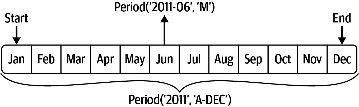
28.5. 기간 연산#

p = pd.Period("2011", freq="A-DEC")
p

Period('2011', 'A-DEC')

p + 5

Period('2016', 'A-DEC')

p - 2

Period('2009', 'A-DEC')

pd.Period("2014", freq="A-DEC") - p

<3 * YearEnds: month=12>

periods = pd.period_range("2000-01-01", "2000-06-30", freq="M")
periods

PeriodIndex(['2000-01', '2000-02', '2000-03', '2000-04', '2000-05', '2000-06'], dtype='period[M]')

pd.Series(np.random.standard_normal(6), index=periods)

2000-01   -0.514551
2000-02   -0.559782
2000-03   -0.783408
2000-04   -1.797685
2000-05   -0.172670
2000-06    0.680215
Freq: M, dtype: float64

values = ["2001Q3", "2002Q2", "2003Q1"]
index = pd.PeriodIndex(values, freq="Q-DEC")
index

PeriodIndex(['2001Q3', '2002Q2', '2003Q1'], dtype='period[Q-DEC]')

28.5.1. 기간 빈도 변환#

p = pd.Period("2011", freq="A-DEC")
p

Period('2011', 'A-DEC')

p.asfreq("M", how="start")

Period('2011-01', 'M')

p.asfreq("M", how="end")

Period('2011-12', 'M')

p.asfreq("M")

Period('2011-12', 'M')

p = pd.Period("2011", freq="A-JUN")
p

Period('2011', 'A-JUN')

p.asfreq("M", how="start")

Period('2010-07', 'M')

p.asfreq("M", how="end")

Period('2011-06', 'M')

<그림 출처: Python for Data Analysis>

p = pd.Period("Aug-2011", "M")
p.asfreq("A-JUN")

Period('2012', 'A-JUN')

periods = pd.period_range("2006", "2009", freq="A-DEC")
ts = pd.Series(np.random.standard_normal(len(periods)), index=periods)
ts

  1.607578
  0.200381
 -0.834068
 -0.302988
Freq: A-DEC, dtype: float64

ts.asfreq("M", how="start")

2006-01    1.607578
2007-01    0.200381
2008-01   -0.834068
2009-01   -0.302988
Freq: M, dtype: float64

ts.asfreq("B", how="end")

2006-12-29    1.607578
2007-12-31    0.200381
2008-12-31   -0.834068
2009-12-31   -0.302988
Freq: B, dtype: float64

28.5.2. 분기 단위 기간#

p = pd.Period("2012Q4", freq="Q-JAN")
p

Period('2012Q4', 'Q-JAN')

p.asfreq("D", how="start")

Period('2011-11-01', 'D')

p.asfreq("D", how="end")

Period('2012-01-31', 'D')

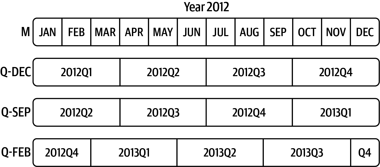
<그림 출처: Python for Data Analysis>

p4pm = (p.asfreq("B", how="end") - 1).asfreq("T", how="start") + 16 * 60
p4pm

Period('2012-01-30 16:00', 'T')

p4pm.to_timestamp()

Timestamp('2012-01-30 16:00:00')

periods = pd.period_range("2011Q3", "2012Q4", freq="Q-JAN")
ts = pd.Series(np.arange(len(periods)), index=periods)
ts

2011Q3    0
2011Q4    1
2012Q1    2
2012Q2    3
2012Q3    4
2012Q4    5
Freq: Q-JAN, dtype: int32

new_periods = (periods.asfreq("B", "end") - 1).asfreq("H", "start") + 16
ts.index = new_periods.to_timestamp()
ts

2010-10-28 16:00:00    0
2011-01-28 16:00:00    1
2011-04-28 16:00:00    2
2011-07-28 16:00:00    3
2011-10-28 16:00:00    4
2012-01-30 16:00:00    5
dtype: int32

28.5.3. 타임 스탬프와 기간#

dates = pd.date_range("2000-01-01", periods=3, freq="M")
ts = pd.Series(np.random.standard_normal(3), index=dates)
ts

2000-01-31    1.663261
2000-02-29   -0.996206
2000-03-31    1.521760
Freq: M, dtype: float64

pts = ts.to_period()
pts

2000-01    1.663261
2000-02   -0.996206
2000-03    1.521760
Freq: M, dtype: float64

dates = pd.date_range("2000-01-29", periods=6)
ts2 = pd.Series(np.random.standard_normal(6), index=dates)
ts2

2000-01-29    0.244175
2000-01-30    0.423331
2000-01-31   -0.654040
2000-02-01    2.089154
2000-02-02   -0.060220
2000-02-03   -0.167933
Freq: D, dtype: float64

ts2.to_period("M")

2000-01    0.244175
2000-01    0.423331
2000-01   -0.654040
2000-02    2.089154
2000-02   -0.060220
2000-02   -0.167933
Freq: M, dtype: float64

pts = ts2.to_period()
pts

2000-01-29    0.244175
2000-01-30    0.423331
2000-01-31   -0.654040
2000-02-01    2.089154
2000-02-02   -0.060220
2000-02-03   -0.167933
Freq: D, dtype: float64

pts.to_timestamp(how="end")

2000-01-29 23:59:59.999999999    0.244175
2000-01-30 23:59:59.999999999    0.423331
2000-01-31 23:59:59.999999999   -0.654040
2000-02-01 23:59:59.999999999    2.089154
2000-02-02 23:59:59.999999999   -0.060220
2000-02-03 23:59:59.999999999   -0.167933
Freq: D, dtype: float64

28.5.4. 기간 인덱스#

base_url = "https://raw.githubusercontent.com/codingalzi/datapy/master/jupyter-book/examples/"
file = "macrodata.csv"

data = pd.read_csv(base_url+file)
data.head(5)

	year	quarter	realgdp	realcons	realinv	realgovt	realdpi	cpi	m1	tbilrate	unemp	pop	infl	realint
0	1959.0	1.0	2710.349	1707.4	286.898	470.045	1886.9	28.98	139.7	2.82	5.8	177.146	0.00	0.00
1	1959.0	2.0	2778.801	1733.7	310.859	481.301	1919.7	29.15	141.7	3.08	5.1	177.830	2.34	0.74
2	1959.0	3.0	2775.488	1751.8	289.226	491.260	1916.4	29.35	140.5	3.82	5.3	178.657	2.74	1.09
3	1959.0	4.0	2785.204	1753.7	299.356	484.052	1931.3	29.37	140.0	4.33	5.6	179.386	0.27	4.06
4	1960.0	1.0	2847.699	1770.5	331.722	462.199	1955.5	29.54	139.6	3.50	5.2	180.007	2.31	1.19

data["year"]

    1959.0
    1959.0
    1959.0
    1959.0
    1960.0
        ...  
  2008.0
  2008.0
  2009.0
  2009.0
  2009.0
Name: year, Length: 203, dtype: float64

data["quarter"]

    1.0
    2.0
    3.0
    4.0
    1.0
      ... 
  3.0
  4.0
  1.0
  2.0
  3.0
Name: quarter, Length: 203, dtype: float64

index = pd.PeriodIndex(year=data["year"], quarter=data["quarter"],
                       freq="Q-DEC")
index

PeriodIndex(['1959Q1', '1959Q2', '1959Q3', '1959Q4', '1960Q1', '1960Q2',
             '1960Q3', '1960Q4', '1961Q1', '1961Q2',
             ...
             '2007Q2', '2007Q3', '2007Q4', '2008Q1', '2008Q2', '2008Q3',
             '2008Q4', '2009Q1', '2009Q2', '2009Q3'],
            dtype='period[Q-DEC]', length=203)

data.index = index
data["infl"]

1959Q1    0.00
1959Q2    2.34
1959Q3    2.74
1959Q4    0.27
1960Q1    2.31
          ... 
2008Q3   -3.16
2008Q4   -8.79
2009Q1    0.94
2009Q2    3.37
2009Q3    3.56
Freq: Q-DEC, Name: infl, Length: 203, dtype: float64

28.6. 리샘플링#

dates = pd.date_range("2000-01-01", periods=100)
ts = pd.Series(np.random.standard_normal(len(dates)), index=dates)
ts

2000-01-01    0.631634
2000-01-02   -1.594313
2000-01-03   -1.519937
2000-01-04    1.108752
2000-01-05    1.255853
                ...   
2000-04-05   -0.423776
2000-04-06    0.789740
2000-04-07    0.937568
2000-04-08   -2.253294
2000-04-09   -1.772919
Freq: D, Length: 100, dtype: float64

ts.resample("M").mean()

2000-01-31   -0.165893
2000-02-29    0.078606
2000-03-31    0.223811
2000-04-30   -0.063643
Freq: M, dtype: float64

ts.resample("M", kind="period").mean()

2000-01   -0.165893
2000-02    0.078606
2000-03    0.223811
2000-04   -0.063643
Freq: M, dtype: float64

28.6.1. 다운 샘플링#

dates = pd.date_range("2000-01-01", periods=12, freq="T")
ts = pd.Series(np.arange(len(dates)), index=dates)
ts

2000-01-01 00:00:00     0
2000-01-01 00:01:00     1
2000-01-01 00:02:00     2
2000-01-01 00:03:00     3
2000-01-01 00:04:00     4
2000-01-01 00:05:00     5
2000-01-01 00:06:00     6
2000-01-01 00:07:00     7
2000-01-01 00:08:00     8
2000-01-01 00:09:00     9
2000-01-01 00:10:00    10
2000-01-01 00:11:00    11
Freq: T, dtype: int32

ts.resample("5min").sum()

2000-01-01 00:00:00    10
2000-01-01 00:05:00    35
2000-01-01 00:10:00    21
Freq: 5T, dtype: int32

ts.resample("5min", closed="right").sum()

1999-12-31 23:55:00     0
2000-01-01 00:00:00    15
2000-01-01 00:05:00    40
2000-01-01 00:10:00    11
Freq: 5T, dtype: int32

ts.resample("5min", closed="right", label="right").sum()

2000-01-01 00:00:00     0
2000-01-01 00:05:00    15
2000-01-01 00:10:00    40
2000-01-01 00:15:00    11
Freq: 5T, dtype: int32

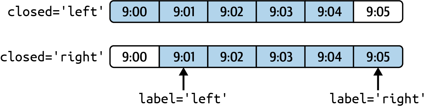
<그림 출처: Python for Data Analysis>

from pandas.tseries.frequencies import to_offset

result = ts.resample("5min", closed="right", label="right").sum()
result.index = result.index + to_offset("-1s")
result

1999-12-31 23:59:59     0
2000-01-01 00:04:59    15
2000-01-01 00:09:59    40
2000-01-01 00:14:59    11
Freq: 5T, dtype: int32

ts = pd.Series(np.random.permutation(np.arange(len(dates))), index=dates)
ts.resample("5min").ohlc()

	open	high	low	close
2000-01-01 00:00:00	8	8	1	5
2000-01-01 00:05:00	6	11	2	2
2000-01-01 00:10:00	0	7	0	7

28.6.2. 업샘플링과 보간법#

frame = pd.DataFrame(np.random.standard_normal((2, 4)),
                     index=pd.date_range("2000-01-01", periods=2,
                                         freq="W-WED"),
                     columns=["Colorado", "Texas", "New York", "Ohio"])
frame

	Colorado	Texas	New York	Ohio
2000-01-05	-0.896431	0.927238	0.482284	-0.867130
2000-01-12	0.493841	-0.155434	1.397286	1.507055

df_daily = frame.resample("D").asfreq()
df_daily

	Colorado	Texas	New York	Ohio
2000-01-05	-0.896431	0.927238	0.482284	-0.867130
2000-01-06	NaN	NaN	NaN	NaN
2000-01-07	NaN	NaN	NaN	NaN
2000-01-08	NaN	NaN	NaN	NaN
2000-01-09	NaN	NaN	NaN	NaN
2000-01-10	NaN	NaN	NaN	NaN
2000-01-11	NaN	NaN	NaN	NaN
2000-01-12	0.493841	-0.155434	1.397286	1.507055

frame.resample("D").ffill()

	Colorado	Texas	New York	Ohio
2000-01-05	-0.896431	0.927238	0.482284	-0.867130
2000-01-06	-0.896431	0.927238	0.482284	-0.867130
2000-01-07	-0.896431	0.927238	0.482284	-0.867130
2000-01-08	-0.896431	0.927238	0.482284	-0.867130
2000-01-09	-0.896431	0.927238	0.482284	-0.867130
2000-01-10	-0.896431	0.927238	0.482284	-0.867130
2000-01-11	-0.896431	0.927238	0.482284	-0.867130
2000-01-12	0.493841	-0.155434	1.397286	1.507055

frame.resample("D").ffill(limit=2)

	Colorado	Texas	New York	Ohio
2000-01-05	-0.896431	0.927238	0.482284	-0.867130
2000-01-06	-0.896431	0.927238	0.482284	-0.867130
2000-01-07	-0.896431	0.927238	0.482284	-0.867130
2000-01-08	NaN	NaN	NaN	NaN
2000-01-09	NaN	NaN	NaN	NaN
2000-01-10	NaN	NaN	NaN	NaN
2000-01-11	NaN	NaN	NaN	NaN
2000-01-12	0.493841	-0.155434	1.397286	1.507055

frame.resample("W-THU").ffill()

	Colorado	Texas	New York	Ohio
2000-01-06	-0.896431	0.927238	0.482284	-0.867130
2000-01-13	0.493841	-0.155434	1.397286	1.507055

28.6.3. 기간 활용 리샘플링#

frame = pd.DataFrame(np.random.standard_normal((24, 4)),
                     index=pd.period_range("1-2000", "12-2001",
                                           freq="M"),
                     columns=["Colorado", "Texas", "New York", "Ohio"])
frame.head()

	Colorado	Texas	New York	Ohio
2000-01	-1.179442	0.443171	1.395676	-0.529658
2000-02	0.787358	0.248845	0.743239	1.267746
2000-03	1.302395	-0.272154	-0.051532	-0.467740
2000-04	-1.040816	0.426419	0.312945	-1.115689
2000-05	1.234297	-1.893094	-1.661605	-0.005477

annual_frame = frame.resample("A-DEC").mean()
annual_frame

	Colorado	Texas	New York	Ohio
2000	0.487329	0.104466	0.020495	-0.273945
2001	0.203125	0.162429	0.056146	-0.103794

# Q-DEC: Quarterly, year ending in December
annual_frame.resample("Q-DEC").ffill()

	Colorado	Texas	New York	Ohio
2000Q1	0.487329	0.104466	0.020495	-0.273945
2000Q2	0.487329	0.104466	0.020495	-0.273945
2000Q3	0.487329	0.104466	0.020495	-0.273945
2000Q4	0.487329	0.104466	0.020495	-0.273945
2001Q1	0.203125	0.162429	0.056146	-0.103794
2001Q2	0.203125	0.162429	0.056146	-0.103794
2001Q3	0.203125	0.162429	0.056146	-0.103794
2001Q4	0.203125	0.162429	0.056146	-0.103794

annual_frame.resample("Q-DEC", convention="end").asfreq()

	Colorado	Texas	New York	Ohio
2000Q4	0.487329	0.104466	0.020495	-0.273945
2001Q1	NaN	NaN	NaN	NaN
2001Q2	NaN	NaN	NaN	NaN
2001Q3	NaN	NaN	NaN	NaN
2001Q4	0.203125	0.162429	0.056146	-0.103794

annual_frame.resample("Q-MAR").ffill()

	Colorado	Texas	New York	Ohio
2000Q4	0.487329	0.104466	0.020495	-0.273945
2001Q1	0.487329	0.104466	0.020495	-0.273945
2001Q2	0.487329	0.104466	0.020495	-0.273945
2001Q3	0.487329	0.104466	0.020495	-0.273945
2001Q4	0.203125	0.162429	0.056146	-0.103794
2002Q1	0.203125	0.162429	0.056146	-0.103794
2002Q2	0.203125	0.162429	0.056146	-0.103794
2002Q3	0.203125	0.162429	0.056146	-0.103794

28.6.4. 시간 리샘플링 그룹화#

N = 15
times = pd.date_range("2017-05-20 00:00", freq="1min", periods=N)
df = pd.DataFrame({"time": times,
                   "value": np.arange(N)})
df

	time	value
0	2017-05-20 00:00:00	0
1	2017-05-20 00:01:00	1
2	2017-05-20 00:02:00	2
3	2017-05-20 00:03:00	3
4	2017-05-20 00:04:00	4
5	2017-05-20 00:05:00	5
6	2017-05-20 00:06:00	6
7	2017-05-20 00:07:00	7
8	2017-05-20 00:08:00	8
9	2017-05-20 00:09:00	9
10	2017-05-20 00:10:00	10
11	2017-05-20 00:11:00	11
12	2017-05-20 00:12:00	12
13	2017-05-20 00:13:00	13
14	2017-05-20 00:14:00	14

df.set_index("time").resample("5min").count()

	value
time
2017-05-20 00:00:00	5
2017-05-20 00:05:00	5
2017-05-20 00:10:00	5

df2 = pd.DataFrame({"time": times.repeat(3),
                    "key": np.tile(["a", "b", "c"], N),
                    "value": np.arange(N * 3.)})
df2.head(7)

	time	key	value
0	2017-05-20 00:00:00	a	0.0
1	2017-05-20 00:00:00	b	1.0
2	2017-05-20 00:00:00	c	2.0
3	2017-05-20 00:01:00	a	3.0
4	2017-05-20 00:01:00	b	4.0
5	2017-05-20 00:01:00	c	5.0
6	2017-05-20 00:02:00	a	6.0

time_key = pd.Grouper(freq="5min")

resampled = (df2.set_index("time")
             .groupby(["key", time_key])
             .sum())
resampled

		value
key	time
a	2017-05-20 00:00:00	30.0
	2017-05-20 00:05:00	105.0
	2017-05-20 00:10:00	180.0
b	2017-05-20 00:00:00	35.0
	2017-05-20 00:05:00	110.0
	2017-05-20 00:10:00	185.0
c	2017-05-20 00:00:00	40.0
	2017-05-20 00:05:00	115.0
	2017-05-20 00:10:00	190.0

resampled.reset_index()

	key	time	value
0	a	2017-05-20 00:00:00	30.0
1	a	2017-05-20 00:05:00	105.0
2	a	2017-05-20 00:10:00	180.0
3	b	2017-05-20 00:00:00	35.0
4	b	2017-05-20 00:05:00	110.0
5	b	2017-05-20 00:10:00	185.0
6	c	2017-05-20 00:00:00	40.0
7	c	2017-05-20 00:05:00	115.0
8	c	2017-05-20 00:10:00	190.0

28.7. 윈도우 함수 활용#

base_url = "https://raw.githubusercontent.com/codingalzi/datapy/master/jupyter-book/examples/"
file = "stock_px.csv"

close_px_all = pd.read_csv(base_url+file, parse_dates=True, index_col=0)
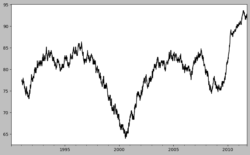
close_px = close_px_all[["AAPL", "MSFT", "XOM"]]
close_px = close_px.resample("B").ffill()

close_px["AAPL"].plot()

<Axes: >

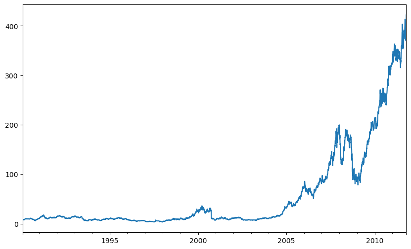
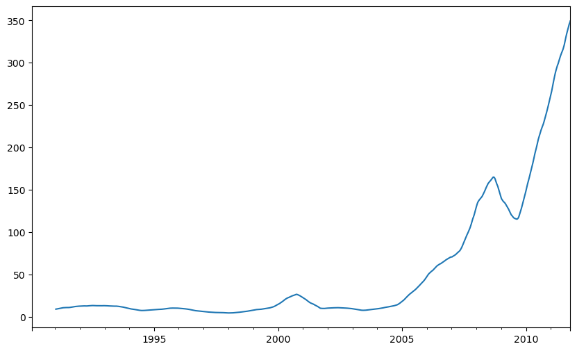
_images/f10464a78f50570d2222a7b0e9f4b434585f427ab86a88afe91952fdb1f48803.png

#! figure,id=apple_daily_ma250,title="Apple price with 250-day moving average"
close_px["AAPL"].rolling(250).mean().plot()

<Axes: >

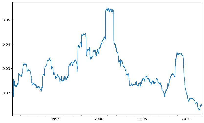
_images/0028cb53d1b21af83f2255e164c2802b1487839f5e18f290087cd9bb6ec4a3e0.png

plt.figure()
std250 = close_px["AAPL"].pct_change().rolling(250, min_periods=10).std()
std250[5:12]
#! figure,id=apple_daily_std250,title="Apple 250-day daily return standard deviation"
std250.plot()

<Axes: >

_images/6c1445e40e88512a3eb1714c2afa82099ba3aece52f61844dd6a181c8f0607b7.png

expanding_mean = std250.expanding().mean()

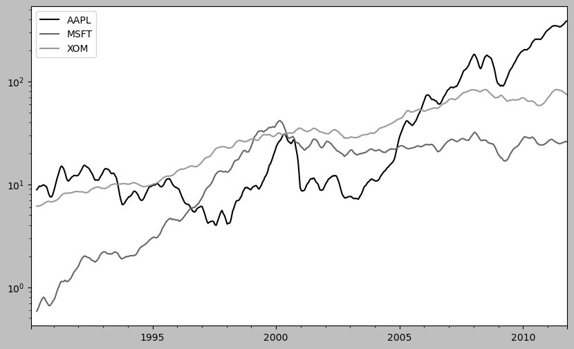
plt.figure()
plt.style.use('grayscale')
#! figure,id=stocks_daily_ma60,title="Stock prices 60-day moving average (log y-axis)"
close_px.rolling(60).mean().plot(logy=True)

<Axes: >

<Figure size 1000x600 with 0 Axes>

_images/18f52b78b51894cf3265877c504729604aec5c4860935ade7bb4f30a0c98f3f0.png

close_px.rolling("20D").mean()

	AAPL	MSFT	XOM
1990-02-01	7.860000	0.510000	6.120000
1990-02-02	7.930000	0.510000	6.180000
1990-02-05	8.013333	0.510000	6.203333
1990-02-06	8.040000	0.510000	6.210000
1990-02-07	7.986000	0.510000	6.234000
...	...	...	...
2011-10-10	389.351429	25.602143	72.527857
2011-10-11	388.505000	25.674286	72.835000
2011-10-12	388.531429	25.810000	73.400714
2011-10-13	388.826429	25.961429	73.905000
2011-10-14	391.038000	26.048667	74.185333

5662 rows × 3 columns

28.7.1. 지수 가중치 함수#

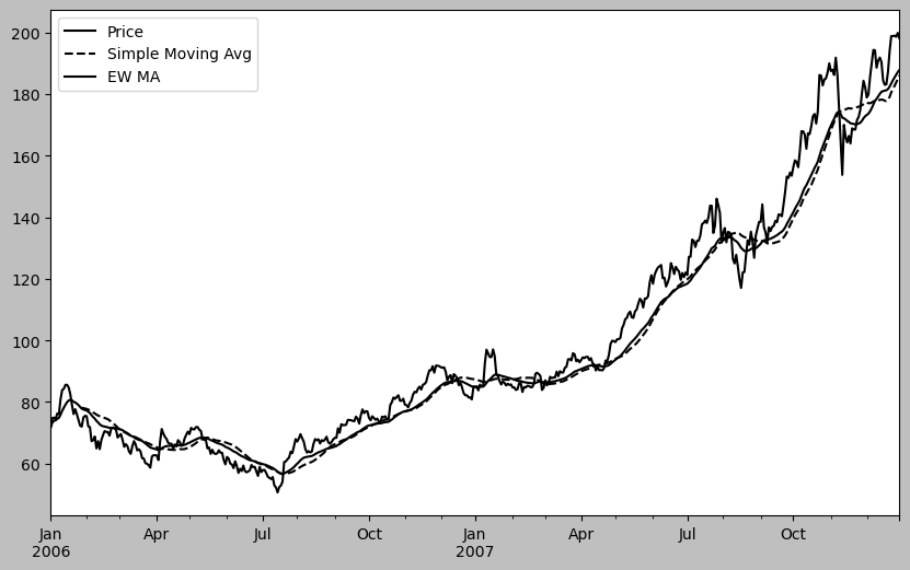
plt.figure()

aapl_px = close_px["AAPL"]["2006":"2007"]

ma30 = aapl_px.rolling(30, min_periods=20).mean()
ewma30 = aapl_px.ewm(span=30).mean()

aapl_px.plot(style="k-", label="Price")
ma30.plot(style="k--", label="Simple Moving Avg")
ewma30.plot(style="k-", label="EW MA")
#! figure,id=timeseries_ewma,title="Simple moving average versus exponentially weighted"
plt.legend()

<matplotlib.legend.Legend at 0x255a3259000>

_images/ba1bd06bab877d1f1b25c91f253a7c6dc1a7ef173ea187e8ec3c974c55b8fbed.png

28.7.2. 이진 이동 윈도우 함수#

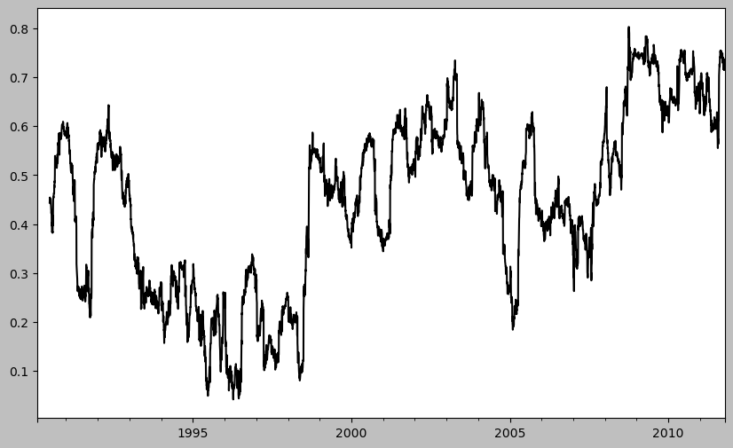
plt.figure()

spx_px = close_px_all["SPX"]
spx_rets = spx_px.pct_change()
returns = close_px.pct_change()

corr = returns["AAPL"].rolling(125, min_periods=100).corr(spx_rets)
#! figure,id=roll_correl_aapl,title="Six-month AAPL return correlation to S&P 500"
corr.plot()

<Axes: >

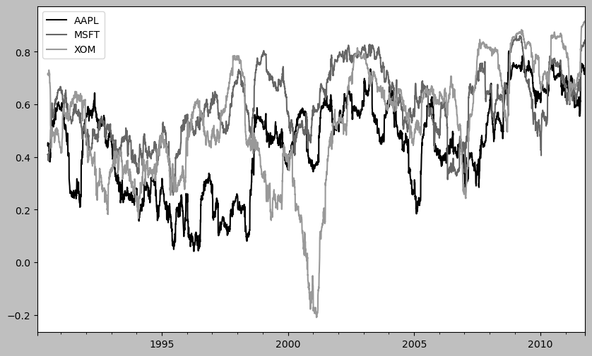
_images/aa172c91b49b23f6068d6aadb87ab5162511e13a55de0c9e93907dd0c0be18eb.png

plt.figure()

corr = returns.rolling(125, min_periods=100).corr(spx_rets)
#! figure,id=roll_correl_all,title="Six-month return correlations to S&P 500"
corr.plot()

<Axes: >

<Figure size 1000x600 with 0 Axes>

_images/f0a988a6deb27cd4039b0fd2b55365f4d6c62b2507675c4db12b9e258cc9a9a3.png

28.7.3. 사용자 정의 윈도우 함수#

plt.figure()

from scipy.stats import percentileofscore
def score_at_2percent(x):
    return percentileofscore(x, 0.02)

result = returns["AAPL"].rolling(250).apply(score_at_2percent)
#! figure,id=roll_apply_ex,title="Percentile rank of 2% AAPL return over one-year window"
result.plot()

<Axes: >

_images/16c6182de6be09fe34795e72bbdc612e06dbba9954378ee5023802631d57805f.png

시계열 데이터

Contents

28. 시계열 데이터#

28.1. datetime 자료형#

28.1.1. 문자열과 Datetime#

28.2. 시계열 데이터 기초#

28.2.1. 인덱싱, 선택, 슬라이싱#

28.2.2. 중복 인덱스 라벨을 갖는 시계열 데이터#

28.3. 날짜 구간 인덱스, 빈도, 시프팅#

28.3.1. 날짜 구간 인덱스 생성#

28.3.2. 빈도와 빈도 단위#

28.3.3. 데이터 시프팅#

28.4. 시간대#

28.4.1. 시간대 지정#

28.4.2. 시간대와 타임 스탬프#

28.4.3. 다른 시간대 다루기#

28.5. 기간 연산#

28.5.1. 기간 빈도 변환#

28.5.2. 분기 단위 기간#

28.5.3. 타임 스탬프와 기간#

28.5.4. 기간 인덱스#

28.6. 리샘플링#

28.6.1. 다운 샘플링#

28.6.2. 업샘플링과 보간법#

28.6.3. 기간 활용 리샘플링#

28.6.4. 시간 리샘플링 그룹화#

28.7. 윈도우 함수 활용#

28.7.1. 지수 가중치 함수#

28.7.2. 이진 이동 윈도우 함수#

28.7.3. 사용자 정의 윈도우 함수#

28.1. `datetime` 자료형#

28.1.1. 문자열과 `Datetime`#