머신러닝 소개 - 실습 - 데이터 과학을 위한 머신러닝

Updated: 17 sep 2026

감사의 글

오렐리앙 제롱Aurélien Géron의 Hands-On Machine Learning with Scikit-Learn and PyTorch (O’Reilly, 2025)에 사용된 코드를 참고한 실습 노트북이다. 보다 심화된 이해를 위해 책 원본을 읽을 것을 강력하게 권장한다. 자료를 공개한 오렐리앙 제롱과 일부 그림 자료를 제공해 준 한빛아카데미에게 진심어린 감사를 전한다.

코드 실행

(구글 코랩) 머신러닝 소개에서 코드를 실행할 수 있다.

환경설정

Python이 3.10 이상의 버전을 요구한다.

import sys

assert sys.version_info >= (3, 10)

Scikit-Learn 라이브러리는 1.6.1 이상의 버전을 요구한다.

from packaging.version import Version
import sklearn

assert Version(sklearn.__version__) >= Version("1.6.1")

그래프에 사용되는 폰트의 크기를 설정한다.

import matplotlib.pyplot as plt

plt.rc('font', size=12)
plt.rc('axes', labelsize=14, titlesize=14)
plt.rc('legend', fontsize=12)
plt.rc('xtick', labelsize=10)
plt.rc('ytick', labelsize=10)

기본 라이브러리

import numpy as np
import pandas as pd

2.1삶의 만족도 예측¶

2.1.1데이터셋 다운로드¶

# Download and prepare the data
data_root = "https://github.com/codingalzi/code-workout-ml/raw/master/notebooks/datasets/"

lifesat_full = pd.read_csv(data_root + "lifesat/lifesat_full.csv")

lifesat_full.set_index("Country", inplace=True)

2020년도 기준 37개 OECD 회원국과 함께 3개 국가가 추가된 총 40개 국가의 데이터로 구성된 데이터프레임이 생성된었음.

lifesat_full.info()

<class 'pandas.DataFrame'>
Index: 40 entries, South Africa to Luxembourg
Data columns (total 2 columns):
 #   Column                Non-Null Count  Dtype  
---  ------                --------------  -----  
 0   GDP per capita (USD)  40 non-null     float64
 1   Life satisfaction     40 non-null     float64
dtypes: float64(2)
memory usage: 1.2 KB

lifesat_full

부분 데이터셋 지정

훈련 데이터가 달라질 때 학습된 모델이 어떻게 달라지는지 비교하기 위해 먼저 일부 데이터만 사용함
먼저 1인당 GDP가 23,500 달러 ~ 62,500 달러 사이의 국가만 선택

gdppc_col = "GDP per capita (USD)"
lifesat_col = "Life satisfaction"

min_gdp = 23_500
max_gdp = 62_500

lifesat = lifesat_full[(lifesat_full[gdppc_col] >= min_gdp) &
                                   (lifesat_full[gdppc_col] <= max_gdp)]

9개 국가가 제외된 총 31개 국가만 선택됨.

lifesat.info()

<class 'pandas.DataFrame'>
Index: 31 entries, Russia to United States
Data columns (total 2 columns):
 #   Column                Non-Null Count  Dtype  
---  ------                --------------  -----  
 0   GDP per capita (USD)  31 non-null     float64
 1   Life satisfaction     31 non-null     float64
dtypes: float64(2)
memory usage: 982.0 bytes

제외된 9개 국가 명단

set(lifesat_full.index) - set(lifesat.index)

{'Brazil',
 'Chile',
 'Colombia',
 'Ireland',
 'Luxembourg',
 'Mexico',
 'Norway',
 'South Africa',
 'Switzerland'}

선택된 31개 국가 산점도

x축: 1인당 GDP
y축: 삶의 만족도
한국 포함 7개 국가 별도 표기.

lifesat.plot(kind='scatter', figsize=(7, 5), grid=True, x=gdppc_col, y=lifesat_col)

position_text = {
    "Turkey": (29_500, 4.2),
    "Hungary": (28_000, 6.9),
    "France": (39_000, 8.0),
    "South Korea": (42_200, 4.5),
    "Australia": (50_000, 5.5),
    "United States": (59_000, 5.3),
    "Denmark": (46_000, 8.5)
}

for country, pos_text in position_text.items():
    pos_data_x = lifesat[gdppc_col].loc[country]
    pos_data_y = lifesat[lifesat_col].loc[country]

    # 미국과 한국 단축명 활용
    if country == "United States":
        country = "US"
    elif  country == "South Korea":
        country = "Korea"
        
    plt.annotate(country, xy=(pos_data_x, pos_data_y),
                 xytext=pos_text, fontsize=12,
                 arrowprops=dict(facecolor='black', width=0.5,
                                 shrink=0.08, headwidth=5))
    plt.plot(pos_data_x, pos_data_y, "ro")


# Set the axis limits
min_life_sat = 4
max_life_sat = 9
plt.axis([min_gdp, max_gdp, min_life_sat, max_life_sat])

plt.show()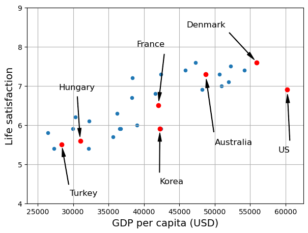

선택된 7개 국가 데이터

highlighted_countries = lifesat.loc[list(position_text.keys())]
highlighted_countries[[gdppc_col, lifesat_col]].sort_values(by=gdppc_col)

적절하지 않은 세 개의 선형 회귀 모델

세 직선의 기울기와 절편은 사람이 수동으로 적절하지 않은 선형 회귀 모델을 시각화하기 위해 임의로 선택됨.

lifesat.plot(kind='scatter', figsize=(7, 5), grid=True, x=gdppc_col, y=lifesat_col)

X_range = np.linspace(min_gdp, max_gdp, 1000)

w1, w2 = 4.2, 0
plt.plot(X_range, w1 + w2 * 1e-5 * X_range, "r")
plt.text(40_000, 4.9, fr"$\theta_0 = {w1}$", color="r")
plt.text(40_000, 4.4, fr"$\theta_1 = {w2}$", color="r")

w1, w2 = 10, -9
plt.plot(X_range, w1 + w2 * 1e-5 * X_range, "g")
plt.text(26_000, 8.5, fr"$\theta_0 = {w1}$", color="g")
plt.text(26_000, 8.0, fr"$\theta_1 = {w2} \times 10^{{-5}}$", color="g")

w1, w2 = 3, 8
plt.plot(X_range, w1 + w2 * 1e-5 * X_range, "b")
plt.text(48_000, 8.5, fr"$\theta_0 = {w1}$", color="b")
plt.text(48_000, 8.0, fr"$\theta_1 = {w2} \times 10^{{-5}}$", color="b")

plt.axis([min_gdp, max_gdp, min_life_sat, max_life_sat])

plt.show()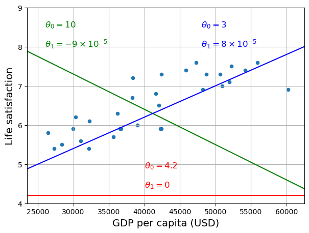

2.1.2선형회귀 예측¶

머신러닝 회귀 모델을 지도학습 방식으로 훈련하려면 훈련에 사용할 특성 데이터 X와 타깃 데이터 y를 지정한다.

특성 데이터 X: 31개 국가의 1인당 GDP
타깃 데이터 y: 31개 국가의 삶의 만족도

훈련셋

X = lifesat[["GDP per capita (USD)"]].values

타깃셋

y = lifesat[["Life satisfaction"]]

선형 회귀 모델 지정

LinearRegression 객체를 생성하여 선형 회귀 모델을 준비한다. 아직 이 단계에서는 데이터로부터 절편과 기울기가 결정되지 않았다. 이를 위해 사이킷런 라이브러리를 다음과 같이 활용한다.

LinearRegression은 sklearn 라이브러리에 포함된 linear_model 모듈에서 정의된 클래스

from sklearn.linear_model import LinearRegression

선형 회귀 모델 지정: LinearRegression 클래스의 객체 생성

# Select a linear model
oecd_linear_model = LinearRegression()

선형 회귀 모델 훈련

훈련셋과 타깃셋을 이용한 지정된 선형 회귀 모델 훈련
fit() 메서드에 훈련셋과 타깃셋을 인자로 지정하여 호출

# Train the model
oecd_linear_model.fit(X, y)

fit()을 호출하면 모델이 훈련되고, 학습된 절편과 계수 등이 모델 객체의 속성에 저장된다.
훈련이 완료된 모델 객체 자체에 저장된 속성(정보)이 달라짐.
예를 들어, 최적의 절편 $\theta_0$ 와 기울기 $\theta_1$ 이 모델 내부에 저장됨.

theta_0, theta_1 = oecd_linear_model.intercept_[0], oecd_linear_model.coef_[0][0]

print(f"theta_0: {theta_0:.2f}")
print(f"theta_1: {theta_1:.2e}")

theta_0: 3.84
theta_1: 6.51e-05

훈련된 모델 활용

oecd_linear_model은 한 국가의 1인당 GDP가 주어졌을 때 해당 국가 국민의 삶의 만족도를 예측하도록 훈련되었다. 훈련된 모델을 이용한 예측은 모델 객체의 predict() 메서드를 활용한다.

모델을 활용한 예측은 훈련할 때 사용된 데이터에 한정되지 않는다. 예를 들어, 아래 코드는 1인당 GDP가 33,422.8 달러인 국가의 국민들의 삶의 만족도는 6.0 정도로 예측된다. 참고로, 33,422.8 달러는 2020년 기준 푸에르토리코의 1인당 GDP이며, 푸에르토리코는 훈련셋에 포함되어 있지 않다.

X_new 변수: predict() 메서드의 인자. 2차원 어레이.

# Make a prediction for Puerto Rico
puerto_rico_gdp_per_capita = 33_442.8  # Puerto Rico' GDP per capita in 2020
X_new = [[puerto_rico_gdp_per_capita]]

puerto_rico_predicted_life_satisfaction = oecd_linear_model.predict(X_new)[0][0]
print(f"푸에르토리코의 2020년 삶의 만족도 예측값: {puerto_rico_predicted_life_satisfaction:.2f}")

푸에르토리코의 2020년 삶의 만족도 예측값: 6.01

모델 훈련으로 정해진 절편과 기울기를 사용하는 1차 함수 $f(x) = \theta_0 + \theta_1 \cdot x$ 를 이용하여 $f(x)$ 를 계산해도 동일한 결과가 나온다.

def f(x):
    return theta_0 + theta_1 * x

f(puerto_rico_gdp_per_capita)

np.float64(6.014985924721082)

predict() 메서드의 인자와 반환값

훈련된 모델의 predict() 메서드에는 일반적으로 2차원 어레이 형태의 입력 데이터를 전달한다. 각 행은 하나의 샘플을, 각 열은 모델이 예측에 사용하는 하나의 특성을 나타낸다.

oecd_linear_model은 한 국가의 삶의 만족도를 예측할 때 해당 국가의 1인당 GDP 하나만을 특성으로 사용한다. 따라서 푸에르토리코의 삶의 만족도를 예측하려면 하나의 샘플에 하나의 특성이 포함된 다음과 같은 2차원 어레이를 입력한다.

[[33442.8]]

여러 국가의 삶의 만족도를 한꺼번에 예측할 때도 같은 원리가 적용된다. 예를 들어 한국과 일본의 1인당 GDP를 이용한다면, 두 국가가 각각 하나의 샘플이 되므로 입력 데이터는 다음과 같이 두 개의 행을 갖는 2차원 어레이가 된다.

[[한국의 1인당 GDP],
 [일본의 1인당 GDP]]

predict() 메서드는 입력된 각 샘플에 대해 하나씩 예측값을 계산한다. 따라서 하나의 타깃인 삶의 만족도를 예측하는 현재 모델에서는 한국과 일본에 대한 두 개의 예측값이 1차원 어레이로 반환된다.

korea_gdp = lifesat_full.loc["South Korea", gdppc_col]
japan_gdp = lifesat_full.loc["Japan", gdppc_col]

print(f"한국 1인당 GDP: {korea_gdp:.2f}")
print(f"일본 1인당 GDP: {japan_gdp}")

print()

print('한국과 일본의 2020년 삶의 만족도 예측값:')
korea_japan_life_satisfaction = oecd_linear_model.predict([[korea_gdp], [japan_gdp]])
print(korea_japan_life_satisfaction)

한국 1인당 GDP: 42251.45
일본 1인당 GDP: 42390.4450571656

한국과 일본의 2020년 삶의 만족도 예측값:
[[6.58802774]
 [6.59707032]]

선형 회귀 예측 그래프

모델이 찾아낸 절편과 기울기를 갖는 직선의 그래프를 데이터 산점도와 함께 그리면 모델이 찾아낸 1인당 GDP와 삶의 만족도 사이의 선형 관계가 매우 적절함을 눈으로 확인할 수 있다. 선형 회귀 모델이 데이터 학습을 통해 어떻게 적절한 절편과 기울기를 학습하는지, 또 그렇게 훈련된 절편과 기울기가 최선인지 여부를 어떻게 판단하는지에 대해서는 앞으로 자세히 다룰 예정이다.

lifesat.plot(kind='scatter', figsize=(7, 5), grid=True, x=gdppc_col, y=lifesat_col)

X_range = np.linspace(min_gdp, max_gdp, 1000)
plt.plot(X_range, theta_0 + theta_1 * X_range, "b")

plt.text(min_gdp + 22_000, max_life_sat - 1.1,
         fr"$\theta_0 = {theta_0:.2f}$", color="b")
plt.text(min_gdp + 22_000, max_life_sat - 0.6,
         fr"$\theta_1 = {theta_1 * 1e5:.2f} \times 10^{{-5}}$", color="b")

plt.axis([min_gdp, max_gdp, min_life_sat, max_life_sat])
plt.show()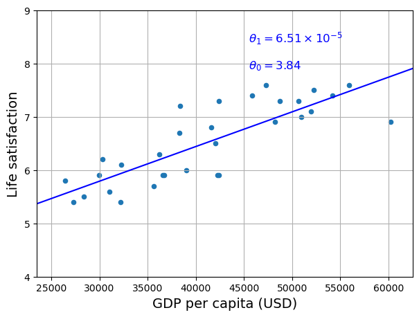

아래 코드는 산점도, 선형 회귀 예측 그래프와 더불어 모델의 훈련에 사용되지 않은 푸에로코리코의 1인당 GDP에 대해 훈련된 모델이 예측한 삶의 만족도를 함께 보여준다.

lifesat.plot(kind='scatter', figsize=(7, 5), grid=True,
                   x=gdppc_col, y=lifesat_col)

X_range = np.linspace(min_gdp, max_gdp, 1000)
plt.plot(X_range, theta_0 + theta_1 * X_range, "b")

plt.text(min_gdp + 22_000, max_life_sat - 1.1,
         fr"$\theta_0 = {theta_0:.2f}$", color="b")
plt.text(min_gdp + 22_000, max_life_sat - 0.6,
         fr"$\theta_1 = {theta_1 * 1e5:.2f} \times 10^{{-5}}$", color="b")

# Plot the prediction for Puerto Rico
plt.plot([puerto_rico_gdp_per_capita, puerto_rico_gdp_per_capita],
         [min_life_sat, puerto_rico_predicted_life_satisfaction], "r--")
plt.text(puerto_rico_gdp_per_capita + 1000, 5.0,
         fr"Prediction = {puerto_rico_predicted_life_satisfaction:.2f}",
         color="r")
plt.plot(puerto_rico_gdp_per_capita, puerto_rico_predicted_life_satisfaction,
         "ro")

plt.axis([min_gdp, max_gdp, min_life_sat, max_life_sat])

plt.show()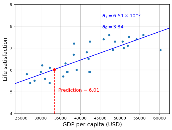

2.2다른 훈련 데이터, 다른 모델¶

이전 모델 훈련에 사용된 훈련셋에서 제외된 국가들의 정보는 다음과 같다.

missing_data = lifesat_full[(lifesat_full[gdppc_col] < min_gdp) |
                            (lifesat_full[gdppc_col] > max_gdp)]
missing_data

2.2.1새로운 선형 회귀 모델¶

제외된 9개 국가를 훈련셋에 포함 시킨 후 새로운 선형 회귀 모델을 훈련시킨다.

훈련셋과 타깃셋

Xfull = np.c_[lifesat_full[gdppc_col]]
yfull = np.c_[lifesat_full[lifesat_col]]

새로운 선형회귀 모델 훈련

from sklearn.linear_model import LinearRegression

oecd_linear_model_full = LinearRegression()
oecd_linear_model_full.fit(Xfull, yfull)

아래 코드는 9개 국가를 제외 했을 때의 선형 회귀 모델(파랑 점선)과 포함시켰을 때의 선형 회귀 모델(검정 실선)의 그래프를 동시에 그린다. 두 모델이 상당히 다름을 확인할 수 있다.

# 40개 국가 산점도
lifesat_full.plot(kind='scatter', figsize=(8, 3),
                        x=gdppc_col, y=lifesat_col, grid=True)

# 9개 국가 주석 추가
position_text_missing_countries = {
    "South Africa": (20_000, 4.2),
    "Colombia": (6_000, 8.2),
    "Brazil": (18_000, 7.8),
    "Mexico": (24_000, 7.4),
    "Chile": (30_000, 7.0),
    "Norway": (51_000, 6.2),
    "Switzerland": (62_000, 5.7),
    "Ireland": (81_000, 5.2),
    "Luxembourg": (92_000, 4.7),
}

for country, pos_text in position_text_missing_countries.items():
    pos_data_x, pos_data_y = missing_data.loc[country]
    plt.annotate(country, xy=(pos_data_x, pos_data_y),
                 xytext=pos_text, fontsize=12,
                 arrowprops=dict(facecolor='black', width=0.5,
                                 shrink=0.08, headwidth=5))
    plt.plot(pos_data_x, pos_data_y, "rs")

# 31개 국가 대상으로 훈련된 선형 회귀 모델
X_range = np.linspace(0, 115_000, 1000)
plt.plot(X_range, theta_0 + theta_1 * X_range, "b:", label="Excluding 9 countries")

# 40개 국가 대상으로 훈련된 선형 회귀 모델
theta_0_full, theta_1_full = oecd_linear_model_full.intercept_[0], oecd_linear_model_full.coef_[0][0]
plt.plot(X_range, theta_0_full + theta_1_full * X_range, "k", label="Incuding 9 countries")

plt.axis([0, 115_000, min_life_sat, max_life_sat])
plt.legend(loc='upper right')
plt.show()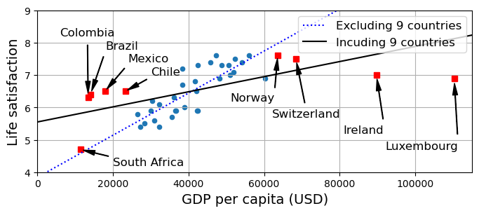

2.2.2선형 회귀 모델 규제¶

릿지(Ridge) 회귀는 선형 회귀 모델의 계수가 지나치게 커지는 것을 제한하는 규제(regularization)가 추가된 선형 회귀 모델이다.

아래에서는 앞에서 사용한 31개 국가의 동일한 데이터에 릿지 회귀를 적용하여 학습된 직선이 어떻게 달라지는지 살펴본다.

from sklearn.linear_model import Ridge

# 릿지 회귀 모델
ridge = Ridge(alpha=10**9.5)

# 훈련셋/타깃셋
X_sample = lifesat[[gdppc_col]]
y_sample = lifesat[[lifesat_col]]

# 릿지 회귀 모델 훈련
ridge.fit(X_sample, y_sample)

아래 그림은 31개 국가만으로 학습한 릿지 회귀 모델(파랑 파선)이 규제를 사용하지 않은 선형 회귀 모델(빨강 점선)보다 기울기가 완만해지고, 40개 국가 전체로 학습한 선형 회귀 모델(검정 실선)에 더 가까운 형태를 보임을 보여준다.

이 그림만으로 릿지 회귀 모델의 예측 성능이 더 좋다고 결론 내릴 수는 없다. 여기서는 규제가 학습된 모델의 형태에 어떤 영향을 줄 수 있는지만 확인한다.

# 9개 국가가 제외된 산점도
lifesat.plot(kind='scatter', x=gdppc_col, y=lifesat_col, figsize=(8, 3))

# 9개 국가 산점도
missing_data.plot(kind='scatter', x=gdppc_col, y=lifesat_col,
                  marker="s", color="r", grid=True, ax=plt.gca())

X_range = np.linspace(0, 115_000, 1000)

# 31개 국가 대상으로 훈련된 선형 회귀 모델
plt.plot(X_range, theta_0 + theta_1*X_range, "b:", label="Linear model on partial data")

# 40개 국가 대상으로 훈련된 선형 회귀 모델
plt.plot(X_range, theta_0_full + theta_1_full * X_range, "k-", label="Linear model on all data")

# 릿지 회귀 모델
theta_0_ridge, theta_1_ridge = ridge.intercept_[0], ridge.coef_[0]
plt.plot(X_range, theta_0_ridge + theta_1_ridge * X_range, "b--",
         label="Regularized linear model on partial data")

plt.legend(loc="lower right")
plt.axis([0, 115_000, min_life_sat, max_life_sat])

plt.show()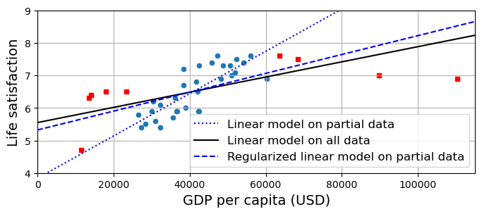

모델 규제에 대해서는 앞으로 자세히 다룰 예정이다.

2.3모델 정리¶

지금까지 사용된 모든 모델의 학습 유형, 과제, 학습 방식, 모델링 방식은 다음과 같다.

학습 유형	과제	학습 방식	모델링 방식
지도학습	회귀	배치 학습	모델 기반

이유는 다음과 같다.

지도학습용 정답 데이터: 국가별 삶의 만족도
회귀 과제: 국가별 삶의 만족도 예측
배치 학습: 삶의 만족도 데이터 전체를 활용한 훈련
모델링 방식: 국가의 1인당 GDP와 삶의 만족도 사이의 관계를 선형 관계로 묘사

2.4부록: OECD 삶의 만족도 데이터셋 생성 과정¶

앞의 실습에서 사용한 lifesat_full.csv 데이터셋이 어떻게 만들어졌는지 살펴본다. 이 절은 머신러닝 모델 학습에 필수적인 내용은 아니며, 원본 데이터를 정리하고 결합하는 과정을 확인하고 싶은 경우 참고한다.

2.4.1데이터 구하기¶

아래 두 사이트에서 다운로드한 파일을 활용하다.

the Better Life Index (BLI) data from OECD’s website (OECD 국가별 삶의 만족도 데이터 포함)
World Bank GDP per capita data from OurWorldInData.org (전세계 국가의 1인당 GDP 데이터 포함)

해당 사이트에서 직접 필요한 파일을 다운로드할 수 있지만 여기서는 아래 코드를 이용하여 두 개의 csv 파일을 다운로드 한다. 만약에 언급된 사이트에서 두 개의 파일을 직접 다운로드한다면 파일 형식이 달라져 있는지 확인한 다음에 필요한 삶의 만족도 데이터 훈련셋을 생성하기 위해 이어지는 코드를 적절히 수정해야 한다.

from pathlib import Path
import urllib.request

datapath = Path() / "datasets" / "lifesat"
datapath.mkdir(parents=True, exist_ok=True)

data_root = "https://github.com/codingalzi/code-workout-ml/raw/master/notebooks/datasets/"
for filename in ("oecd_bli.csv", "gdp_per_capita.csv"):
    if not (datapath / filename).is_file():
        print("Downloading", filename)
        url = data_root + "lifesat/" + filename
        urllib.request.urlretrieve(url, datapath / filename)

oecd_bli = pd.read_csv(datapath / "oecd_bli.csv")
gdp_per_capita = pd.read_csv(datapath / "gdp_per_capita.csv")

oecd_bli.info()

<class 'pandas.DataFrame'>
RangeIndex: 2369 entries, 0 to 2368
Data columns (total 17 columns):
 #   Column                 Non-Null Count  Dtype  
---  ------                 --------------  -----  
 0   LOCATION               2369 non-null   str    
 1   Country                2369 non-null   str    
 2   INDICATOR              2369 non-null   str    
 3   Indicator              2369 non-null   str    
 4   MEASURE                2369 non-null   str    
 5   Measure                2369 non-null   str    
 6   INEQUALITY             2369 non-null   str    
 7   Inequality             2369 non-null   str    
 8   Unit Code              2369 non-null   str    
 9   Unit                   2369 non-null   str    
 10  PowerCode Code         2369 non-null   int64  
 11  PowerCode              2369 non-null   str    
 12  Reference Period Code  0 non-null      float64
 13  Reference Period       0 non-null      float64
 14  Value                  2369 non-null   float64
 15  Flag Codes             0 non-null      float64
 16  Flags                  0 non-null      float64
dtypes: float64(5), int64(1), str(11)
memory usage: 478.8 KB

oecd_bli

gdp_per_capita.info()

<class 'pandas.DataFrame'>
RangeIndex: 7110 entries, 0 to 7109
Data columns (total 4 columns):
 #   Column                                               Non-Null Count  Dtype  
---  ------                                               --------------  -----  
 0   Entity                                               7110 non-null   str    
 1   Code                                                 5730 non-null   str    
 2   Year                                                 7110 non-null   int64  
 3   GDP per capita, PPP (constant 2017 international $)  7110 non-null   float64
dtypes: float64(1), int64(1), str(2)
memory usage: 320.4 KB

gdp_per_capita

2.4.2데이터 전처리¶

2020년 기준 1인당 GDP 데이터 추출

gdp_year = 2020
gdppc_col = "GDP per capita (USD)"
lifesat_col = "Life satisfaction"

gdp_per_capita = gdp_per_capita[gdp_per_capita["Year"] == gdp_year]
gdp_per_capita = gdp_per_capita.drop(["Code", "Year"], axis=1)
gdp_per_capita.columns = ["Country", gdppc_col]
gdp_per_capita.set_index("Country", inplace=True)

gdp_per_capita

앞서 언급된 푸에르토리코의 1인당 GDP 정보는 다음과 같이 구한다.

puerto_rico_gdp_per_capita = gdp_per_capita[gdppc_col].loc["Puerto Rico"]
puerto_rico_gdp_per_capita

np.float64(33442.8315702748)

삶의 만족도(Life satisfaction) 데이터 추출

oecd_bli = oecd_bli[oecd_bli["INEQUALITY"]=="TOT"]
oecd_bli = oecd_bli.pivot(index="Country", columns="Indicator", values="Value")

oecd_bli

oecd_bli_list = oecd_bli.index.tolist()
gdp_per_capita_list = gdp_per_capita.index.tolist()

두 데이터셋의 인덱스로 사용된 국가명 차이 확인

set(oecd_bli_list) - set(gdp_per_capita_list)

{'Czech Republic', 'Korea', 'OECD - Total', 'Slovak Republic'}

'OECD - Total'은 국가가 아님. 삭제 대상

oecd_bli.drop(index=['OECD - Total'], inplace=True)

체코, 대한민국, 슬로바키아 세 나라의 국가명이 두 데이터셋에서 다르게 불림. 이름 통일 필요.
- oecd_bli.csv 파일: Czech Repulic, Korea, Slovak Republic
- gdp_per_capita.csv 파일: Czechia, South Korea, Slovakia

names_to_change = {'Czech Republic': 'Czechia',
                   'Korea': 'South Korea',
                   'Slovak Republic': 'Slovakia'}

oecd_bli.rename(index=names_to_change, inplace=True)

수정 결과 확인

oecd_bli_list = oecd_bli.index.tolist()
gdp_per_capita_list = gdp_per_capita.index.tolist()

set(oecd_bli_list) - set(gdp_per_capita_list)

set()

1인당 GDP 데이터와 삶이 만족도 데이터 병합

full_country_stats = pd.merge(left=oecd_bli, right=gdp_per_capita,
                              left_index=True, right_index=True)
full_country_stats.sort_values(by=gdppc_col, inplace=True)
full_country_stats = full_country_stats[[gdppc_col, lifesat_col]]

full_country_stats

최종 데이터셋 파일 저장

full_country_stats.to_csv(datapath / "lifesat_full.csv")

2 머신러닝 소개 - 실습