감사의 글
아래 내용은 프랑소와 숄레의 Deep Learning with Python(3판)의 소스코드 내용을 참고해서 작성되었습니다. 자료를 공개한 저자에게 진심어린 감사를 전합니다.
코드 실행
(구글 코랩) P3 실습: 합성곱 신경망과 컴퓨터 비전에서 코드를 실행할 수 있다.
주요 내용
MNIST를 CNN으로 분류하고 합성곱·풀링·특성맵을 관찰한다.
Keras와 PyTorch로 동일한 CNN 개념을 표현한다.
작은 이미지 데이터셋에서 데이터 증식과 전이 학습을 비교한다.
이미지 분류를 넘어 객체 탐지 문제를 살펴본다.
잔차 연결, 배치 정규화, 채널 분리 합성곱을 간단한 코드로 확인한다.
설정: TensorFlow와 Keras의 GPU 사용 가능 여부 확인
# TensorFlow 를 사용할 때 기타 정보 표시 제한. Tensorflow를 불러오기 전에 실행해야 함
import os
os.environ["TF_CPP_MIN_LOG_LEVEL"] = "2"

import tensorflow as tf
import torch

# TensorFlow
tf_gpus = tf.config.list_physical_devices("GPU")

print("=== TensorFlow ===")
print("Version:", tf.__version__)
print("GPU 사용 가능:", len(tf_gpus) > 0)
if tf_gpus:
    print("GPU:", tf_gpus[0].name)

print()

# PyTorch
print("=== PyTorch ===")
print("Version:", torch.__version__)
print("GPU 사용 가능:", torch.cuda.is_available())
if torch.cuda.is_available():
    print("GPU:", torch.cuda.get_device_name(0))
    print("CUDA version:", torch.version.cuda)
=== TensorFlow ===
Version: 2.20.0
GPU 사용 가능: True
GPU: /physical_device:GPU:0
=== PyTorch ===
Version: 2.9.1+cu128
GPU 사용 가능: True
GPU: NVIDIA RTX A6000
CUDA version: 12.8
필수 라이브러리
import numpy as np
import matplotlib.pyplot as plt
import keras
from keras import layers10.1MNIST: 이미지를 펼치지 않고 분류하기
10.1.1입력 구조 확인
MLP는 (28, 28) 이미지를 784개의 값으로 펼쳐 입력할 수 있다. CNN은 높이와 너비, 채널의 구분을 유지한다. 흑백 이미지에는 채널이 1개 있다.
from keras.datasets import mnist

(mnist_x_all, mnist_y_all), (mnist_x_test, mnist_y_test) = mnist.load_data()

mnist_x_all = mnist_x_all.astype("float32")[..., None] / 255.0
mnist_x_test = mnist_x_test.astype("float32")[..., None] / 255.0

rng = np.random.default_rng(42)
order = rng.permutation(len(mnist_x_all))
n_val = int(len(mnist_x_all) * 0.10)
train_ids, val_ids = order[:-n_val], order[-n_val:]

mnist_x_train, mnist_y_train = mnist_x_all[train_ids], mnist_y_all[train_ids]
mnist_x_val, mnist_y_val = mnist_x_all[val_ids], mnist_y_all[val_ids]

print("훈련:", mnist_x_train.shape, mnist_y_train.shape)
print("검증:", mnist_x_val.shape, mnist_y_val.shape)
print("테스트:", mnist_x_test.shape, mnist_y_test.shape)
훈련: (54000, 28, 28, 1) (54000,)
검증: (6000, 28, 28, 1) (6000,)
테스트: (10000, 28, 28, 1) (10000,)
관찰: MNIST의 훈련용 이미지 60,000개를 모두 사용한다. 이 중 54,000개는 모델 훈련에, 6,000개는 검증에 배정했다. 각 샘플은 (28, 28, 1)이며 마지막 1은 흑백 이미지의 채널 수다. 별도의 테스트 이미지 10,000개는 마지막 평가 때만 사용한다.
fig, axes = plt.subplots(1, 5, figsize=(10, 2))
for i, ax in enumerate(axes):
    ax.imshow(mnist_x_train[i, :, :, 0], cmap="gray")
    ax.set_title(f"Label: {mnist_y_train[i]}")
    ax.axis("off")
plt.tight_layout()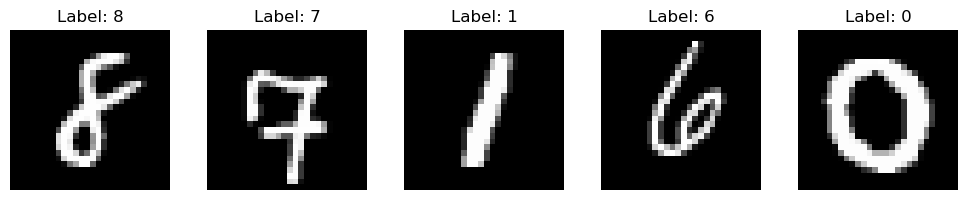
10.1.2Keras CNN 모델 만들기
합성곱 층 → 맥스 풀링 층을 반복한 다음 분류 출력층을 연결한다. 이미지의 공간 정보를 보존하는 것이 MLP와 가장 큰 차이다.
inputs = keras.Input(shape=(28, 28, 1))
x = layers.Conv2D(32, 3, padding="same", activation="relu", name="first_conv")(inputs)
x = layers.MaxPooling2D(pool_size=2)(x)
x = layers.Conv2D(64, 3, padding="same", activation="relu")(x)
x = layers.MaxPooling2D(pool_size=2)(x)
x = layers.Conv2D(128, 3, padding="same", activation="relu")(x)
x = layers.GlobalAveragePooling2D()(x)
outputs = layers.Dense(10, activation="softmax")(x)

mnist_cnn = keras.Model(inputs, outputs, name="mnist_cnn")
mnist_cnn.summary()
WARNING: All log messages before absl::InitializeLog() is called are written to STDERR
I0000 00:00:1794293928.968011 19481 gpu_device.cc:2020] Created device /job:localhost/replica:0/task:0/device:GPU:0 with 46007 MB memory: -> device: 0, name: NVIDIA RTX A6000, pci bus id: 0000:01:00.0, compute capability: 8.6
Conv2D(32, 3)은 3×3 커널을 가진 필터 32개를 사용한다. 따라서 출력 채널 수는 32다. MaxPooling2D(2)는 각 채널의 높이와 너비를 줄이고, GlobalAveragePooling2D는 채널마다 평균값 하나를 만든다.
확인: summary()에서 공간 크기는 작아지고 채널 수는 커지는지 살펴보자.
10.1.3훈련·검증 곡선 확인
다중 클래스 분류이므로 정수 타깃에는 sparse_categorical_crossentropy를 사용한다. 정확도 하나만 보지 말고, 훈련·검증 곡선이 어떻게 다른지도 확인한다.
mnist_cnn.compile(
    optimizer="adam",
    loss="sparse_categorical_crossentropy",
    metrics=["accuracy"],
)

mnist_history = mnist_cnn.fit(
    mnist_x_train, mnist_y_train,
    validation_data=(mnist_x_val, mnist_y_val),
    epochs=4, batch_size=128, verbose=1,
)
Epoch 1/4
68/422 ━━━━━━━━━━━━━━━━━━━━ 0s 2ms/step - accuracy: 0.1618 - loss: 2.2155I0000 00:00:1794293932.949287 19663 device_compiler.h:196] Compiled cluster using XLA! This line is logged at most once for the lifetime of the process.
422/422 ━━━━━━━━━━━━━━━━━━━━ 0s 5ms/step - accuracy: 0.5269 - loss: 1.36532026-11-10 15:58:57.107827: E external/local_xla/xla/service/slow_operation_alarm.cc:73] Trying algorithm eng33{k2=2,k6=0,k13=2,k14=0,k22=1} for conv (f32[112,64,14,14]{3,2,1,0}, u8[0]{0}) custom-call(f32[112,32,14,14]{3,2,1,0}, f32[64,32,3,3]{3,2,1,0}, f32[64]{0}), window={size=3x3 pad=1_1x1_1}, dim_labels=bf01_oi01->bf01, custom_call_target="__cudnn$convBiasActivationForward", backend_config={"operation_queue_id":"0","wait_on_operation_queues":[],"cudnn_conv_backend_config":{"activation_mode":"kRelu","conv_result_scale":1,"side_input_scale":0,"leakyrelu_alpha":0},"force_earliest_schedule":false,"reification_cost":[]} is taking a while...
2026-11-10 15:58:57.109294: E external/local_xla/xla/service/slow_operation_alarm.cc:140] The operation took 1.518006545s
Trying algorithm eng33{k2=2,k6=0,k13=2,k14=0,k22=1} for conv (f32[112,64,14,14]{3,2,1,0}, u8[0]{0}) custom-call(f32[112,32,14,14]{3,2,1,0}, f32[64,32,3,3]{3,2,1,0}, f32[64]{0}), window={size=3x3 pad=1_1x1_1}, dim_labels=bf01_oi01->bf01, custom_call_target="__cudnn$convBiasActivationForward", backend_config={"operation_queue_id":"0","wait_on_operation_queues":[],"cudnn_conv_backend_config":{"activation_mode":"kRelu","conv_result_scale":1,"side_input_scale":0,"leakyrelu_alpha":0},"force_earliest_schedule":false,"reification_cost":[]} is taking a while...
422/422 ━━━━━━━━━━━━━━━━━━━━ 7s 10ms/step - accuracy: 0.7442 - loss: 0.7905 - val_accuracy: 0.9175 - val_loss: 0.2856
Epoch 2/4
422/422 ━━━━━━━━━━━━━━━━━━━━ 1s 2ms/step - accuracy: 0.9316 - loss: 0.2326 - val_accuracy: 0.9253 - val_loss: 0.2356
Epoch 3/4
422/422 ━━━━━━━━━━━━━━━━━━━━ 1s 2ms/step - accuracy: 0.9491 - loss: 0.1669 - val_accuracy: 0.9615 - val_loss: 0.1360
Epoch 4/4
422/422 ━━━━━━━━━━━━━━━━━━━━ 1s 2ms/step - accuracy: 0.9590 - loss: 0.1352 - val_accuracy: 0.9578 - val_loss: 0.1371
fig, axes = plt.subplots(1, 2, figsize=(10, 3.5))

for key, title, ax in [("loss", "Loss", axes[0]), ("accuracy", "Accuracy", axes[1])]:
    epochs = range(1, len(mnist_history.history[key]) + 1)
    ax.plot(epochs, mnist_history.history[key], label="Train")
    ax.plot(epochs, mnist_history.history["val_" + key], label="Validation")
    ax.set_xlabel("Epoch")
    ax.set_xticks(range(1, 5))
    ax.set_title(title)
    ax.legend()

plt.tight_layout()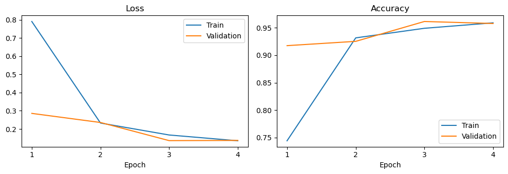
생각해보기: 훈련 손실이 감소하는데 검증 손실은 더 이상 감소하지 않는다면 무엇을 의심해야 할까? 모델 성능을 개선하려면 어떤 데이터를 기준으로 판단해야 할까?
10.1.4채널 수와 파라미터 수 비교
필터 수는 출력 채널 수를 결정한다. 필터의 크기와 입력 채널 수는 합성곱 층에 필요한 가중치 수에 영향을 준다. 같은 공간 크기를 다루더라도 Dense 층과 합성곱 층의 파라미터 수는 크게 다를 수 있다.
conv_example = layers.Conv2D(32, 3, use_bias=False)
conv_example(keras.Input(shape=(28, 28, 1)))

dense_example = layers.Dense(32, use_bias=False)
dense_example(keras.Input(shape=(28*28,)))

print("Conv2D 파라미터:", conv_example.count_params())
print("Dense 파라미터:", dense_example.count_params())
Conv2D 파라미터: 288
Dense 파라미터: 25088
10.2PyTorch로 같은 CNN 구성하기
Keras와 PyTorch는 서로 다른 신경망 원리가 아니다. 다만 이미지 텐서의 채널 축 위치와 훈련 방식이 다르다.
Keras:
(배치, 높이, 너비, 채널)— NHWCPyTorch:
(배치, 채널, 높이, 너비)— NCHW
PyTorch의 nn.CrossEntropyLoss는 logits를 입력으로 받으므로 모델의 마지막 층에 Softmax를 추가하지 않는다.
from torch import nn
from torch.utils.data import TensorDataset, DataLoader

device = torch.device("cuda" if torch.cuda.is_available() else "cpu")
print("장치:", device)

torch_x_train = torch.from_numpy(mnist_x_train).permute(0, 3, 1, 2)
torch_x_val = torch.from_numpy(mnist_x_val).permute(0, 3, 1, 2)
torch_x_test = torch.from_numpy(mnist_x_test).permute(0, 3, 1, 2)

train_loader = DataLoader(TensorDataset(torch_x_train, torch.from_numpy(mnist_y_train).long()),
                          batch_size=128, shuffle=True)
val_loader = DataLoader(TensorDataset(torch_x_val, torch.from_numpy(mnist_y_val).long()),
                        batch_size=256)
test_loader = DataLoader(TensorDataset(torch_x_test, torch.from_numpy(mnist_y_test).long()),
                         batch_size=256)

print("Keras 첫 배치 차원:", mnist_x_train[:128].shape)
print("PyTorch 첫 배치 차원:", next(iter(train_loader))[0].shape)
장치: cuda
Keras 첫 배치 차원: (128, 28, 28, 1)
PyTorch 첫 배치 차원: torch.Size([128, 1, 28, 28])
10.2.1forward()에서 층을 직접 연결하기
모델의 층은 __init__()에서 정의하고, forward()에서 계산 순서를 명시한다.
class TorchMNISTCNN(nn.Module):
    def __init__(self):
        super().__init__()
        self.conv1 = nn.Conv2d(1, 32, 3, padding=1)
        self.conv2 = nn.Conv2d(32, 64, 3, padding=1)
        self.conv3 = nn.Conv2d(64, 128, 3, padding=1)
        self.pool = nn.MaxPool2d(2)
        self.relu = nn.ReLU()
        self.gap = nn.AdaptiveAvgPool2d(1)
        self.output = nn.Linear(128, 10)

    def forward(self, x):
        x = self.pool(self.relu(self.conv1(x)))
        x = self.pool(self.relu(self.conv2(x)))
        x = self.relu(self.conv3(x))
        x = self.gap(x)
        x = torch.flatten(x, start_dim=1)
        return self.output(x)  # logits

torch_cnn = TorchMNISTCNN().to(device)
print(torch_cnn)
TorchMNISTCNN(
(conv1): Conv2d(1, 32, kernel_size=(3, 3), stride=(1, 1), padding=(1, 1))
(conv2): Conv2d(32, 64, kernel_size=(3, 3), stride=(1, 1), padding=(1, 1))
(conv3): Conv2d(64, 128, kernel_size=(3, 3), stride=(1, 1), padding=(1, 1))
(pool): MaxPool2d(kernel_size=2, stride=2, padding=0, dilation=1, ceil_mode=False)
(relu): ReLU()
(gap): AdaptiveAvgPool2d(output_size=1)
(output): Linear(in_features=128, out_features=10, bias=True)
)
10.2.2훈련과 검증
PyTorch에서는 zero_grad() → forward → loss → backward() → step()을 직접 작성한다. 검증 때는 eval()로 모드를 바꾸고 기울기 계산을 끈다.
def run_torch_epoch(model, loader, loss_fn, optimizer=None):
    training = optimizer is not None
    model.train() if training else model.eval()
    total_loss, correct, total = 0.0, 0, 0

    with torch.set_grad_enabled(training):
        for xb, yb in loader:
            xb, yb = xb.to(device), yb.to(device)
            if training:
                optimizer.zero_grad()
            logits = model(xb)
            loss = loss_fn(logits, yb)
            if training:
                loss.backward()
                optimizer.step()
            total_loss += loss.item() * len(xb)
            correct += (logits.argmax(dim=1) == yb).sum().item()
            total += len(xb)
    return total_loss / total, correct / total

loss_fn = nn.CrossEntropyLoss()
optimizer = torch.optim.Adam(torch_cnn.parameters(), lr=1e-3)

torch_history = {"loss": [], "accuracy": [], "val_loss": [], "val_accuracy": []}
for epoch in range(3):
    tr_loss, tr_acc = run_torch_epoch(torch_cnn, train_loader, loss_fn, optimizer)
    va_loss, va_acc = run_torch_epoch(torch_cnn, val_loader, loss_fn)
    for key, value in [("loss", tr_loss), ("accuracy", tr_acc),
                       ("val_loss", va_loss), ("val_accuracy", va_acc)]:
        torch_history[key].append(value)
    print(f"epoch {epoch+1}: loss={tr_loss:.3f}, accuracy={tr_acc:.3f}, "
          f"val_loss={va_loss:.3f}, val_accuracy={va_acc:.3f}")
epoch 1: loss=1.023, accuracy=0.666, val_loss=0.355, val_accuracy=0.901
epoch 2: loss=0.281, accuracy=0.917, val_loss=0.219, val_accuracy=0.939
epoch 3: loss=0.203, accuracy=0.940, val_loss=0.167, val_accuracy=0.953
검증: 같은 CNN 개념으로 모델을 구성했지만 두 프레임워크의 결과가 정확히 같을 필요는 없다. 초기 가중치와 훈련 방식 등이 다르기 때문이다. 비교할 때는 사용한 데이터와 평가 기준을 먼저 확인한다.
10.2.3MNIST 테스트 데이터에서 최종 평가
훈련과 검증을 마친 후에만 테스트 데이터로 평가한다. 테스트 결과를 보고 모델을 반복해서 수정하면 테스트 데이터가 사실상 검증 데이터처럼 사용된다.
keras_test_loss, keras_test_acc = mnist_cnn.evaluate(mnist_x_test, mnist_y_test, verbose=0)
torch_test_loss, torch_test_acc = run_torch_epoch(torch_cnn, test_loader, loss_fn)
print(f"Keras    테스트 정확도: {keras_test_acc:.3f}")
print(f"PyTorch  테스트 정확도: {torch_test_acc:.3f}")
Keras 테스트 정확도: 0.959
PyTorch 테스트 정확도: 0.954
10.3작은 이미지 데이터셋: 고양이와 개 분류
CIFAR-10 데이터셋에 포함된 이미지에서 고양이(cat)와 개(dog) 두 클래스만 추출하여 이진 분류 문제를 만든다. 이를 통해 CNN 기준 모델과 데이터 증식, 전이 학습을 비교한다.
CIFAR-10 이미지는 32×32 픽셀로 매우 작다. 이미지 해상도와 데이터의 특성이 모델 성능에 영향을 줄 수 있다.
주의: 아래 코드를 실행하면 “Widgets require us to download supporting files from a 3rd party website.” 라는 경고문과 함께 다운로드를 계속 진행할지 여부를 묻는다. 이는 Hugging Fase에서 데이터셋을 다운로드할 때 다운로드 진행률을 보여주는 위젯의 작동에 대한 경고문이며 “Enable Downloads” 버튼을 누르면 아무 문제없이 데이터셋이 다운로드 된다.
import numpy as np
from datasets import load_dataset

# --------------------------------------------------
# 1. CIFAR-10 데이터셋 불러오기
# --------------------------------------------------

# Hugging Face에서 CIFAR-10 다운로드
# train: 50,000장 / test: 10,000장
# 각 이미지는 32×32 크기의 RGB 이미지
cifar = load_dataset("uoft-cs/cifar10")

# 이미지의 클래스 번호(label)만 NumPy 배열로 변환
cifar_y_train_all = np.array(cifar["train"]["label"])
cifar_y_test_all = np.array(cifar["test"]["label"])


# --------------------------------------------------
# 2. 고양이(cat)와 개(dog) 이미지 선택
# --------------------------------------------------

# CIFAR-10 클래스 번호: cat=3, dog=5
# 이진 분류 타깃: cat=0, dog=1

# 난수 시드를 고정하여 동일한 데이터 선택을 재현
rng = np.random.default_rng(42)

# 훈련, 검증, 테스트 이미지의 인덱스를 저장할 리스트
train_ids, val_ids, test_ids = [], [], []

# 고양이(3)와 개(5)를 각각 같은 수만큼 선택
for original_class in (3, 5):

    # 해당 클래스에 속한 이미지의 인덱스를 찾아 무작위로 섞기
    tr = rng.permutation(
        np.flatnonzero(cifar_y_train_all == original_class)
    )
    te = rng.permutation(
        np.flatnonzero(cifar_y_test_all == original_class)
    )

    # 원래 훈련 데이터에서 클래스별 1,000장씩 선택
    train_ids.extend(tr[:1000])

    # 원래 훈련 데이터에서 클래스별 250장씩 검증용으로 선택
    val_ids.extend(tr[1000:1250])

    # 원래 테스트 데이터에서 클래스별 300장씩 선택
    test_ids.extend(te[:300])

# 고양이와 개 이미지가 섞이도록 전체 순서를 다시 무작위로 변경
train_ids = rng.permutation(train_ids)
val_ids = rng.permutation(val_ids)
test_ids = rng.permutation(test_ids)


# --------------------------------------------------
# 3. 선택한 이미지만 NumPy 배열로 변환
# --------------------------------------------------

def get_images(split, ids):
    """선택된 이미지들을 float32 NumPy 배열로 반환"""

    # split: "train" 또는 "test"
    # ids: 선택할 이미지의 인덱스
    # 각 이미지를 NumPy 배열로 바꾼 뒤 하나의 배열로 결합
    return np.stack([
        np.array(cifar[split][int(i)]["img"], dtype="float32")
        for i in ids
    ])


# --------------------------------------------------
# 4. 훈련·검증·테스트 데이터 생성
# --------------------------------------------------

# 훈련 데이터
catdog_x_train = get_images("train", train_ids)
catdog_y_train = (cifar_y_train_all[train_ids] == 5).astype("float32")

# 검증 데이터: 원래 훈련 데이터에서 분리
catdog_x_val = get_images("train", val_ids)
catdog_y_val = (cifar_y_train_all[val_ids] == 5).astype("float32")

# 테스트 데이터: 원래 테스트 데이터에서 선택
catdog_x_test = get_images("test", test_ids)
catdog_y_test = (cifar_y_test_all[test_ids] == 5).astype("float32")

# 레이블 변환 원리:
# cat(3) == 5 → False → 0.0
# dog(5) == 5 → True  → 1.0

# 주의: 이미지를 float32로 변환했지만 픽셀값은 여전히
# 0~255 범위이다. 정규화·모델별 전처리는 이후 단계에서 수행한다.


# --------------------------------------------------
# 5. 데이터 구성 결과 확인
# --------------------------------------------------

print("훈련 / 검증 / 테스트:",
      len(train_ids), len(val_ids), len(test_ids))

print("훈련 이미지:", catdog_x_train.shape)
print("검증 이미지:", catdog_x_val.shape)
print("테스트 이미지:", catdog_x_test.shape)
print("이미지 모양:", catdog_x_train.shape[1:])훈련 / 검증 / 테스트: 2000 500 600
훈련 이미지: (2000, 32, 32, 3)
검증 이미지: (500, 32, 32, 3)
테스트 이미지: (600, 32, 32, 3)
이미지 모양: (32, 32, 3)
고양이와 개 중 하나를 예측하는 이진 분류다. 따라서 출력 유닛 하나와 Sigmoid, 이진 교차엔트로피를 사용할 수 있다. 이미지의 해상도가 작으므로 작은 CNN으로 먼저 기준 모델을 만든다.
fig, axes = plt.subplots(2, 5, figsize=(9, 4))
for ax, image, label in zip(axes.flat, catdog_x_train[:10], catdog_y_train[:10]):
    ax.imshow(image.astype("uint8"))
    ax.set_title("dog" if label == 1 else "cat")
    ax.axis("off")
plt.tight_layout()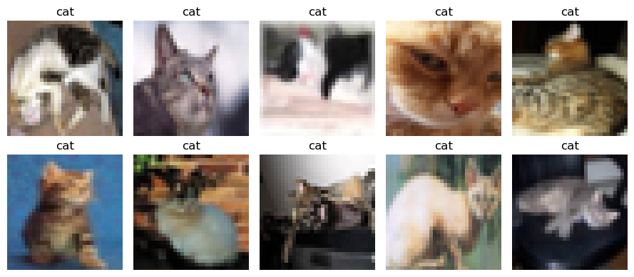
10.3.1기준 CNN과 데이터 증식 CNN 비교
데이터 증식(augmentation)은 훈련 이미지를 반전·회전 등으로 조금씩 바꾸어 모델이 특정 사진에만 의존하지 않도록 돕는다. 타깃의 의미를 보존하는 변환이어야 한다. 데이터 증식은 별도의 실제 사진을 새로 수집하는 것과는 다르다.
augmentation = keras.Sequential([
    layers.RandomFlip("horizontal"),
    layers.RandomRotation(0.10),
    layers.RandomTranslation(0.10, 0.10),
    layers.RandomZoom(0.07),
    layers.RandomContrast(0.5),
], name="augmentation")

image = catdog_x_train[:1]

fig, axes = plt.subplots(2, 5, figsize=(9, 4))
axes = axes.flatten()

axes[0].imshow(image[0].astype("uint8"))
axes[0].set_title("Original")

for i, ax in enumerate(axes[1:], start=1):
    changed = augmentation(image, training=True).numpy()[0]
    ax.imshow(np.clip(changed, 0, 255).astype("uint8"))
    ax.set_title(f"Augmented {i}")

for ax in axes:
    ax.axis("off")

plt.tight_layout()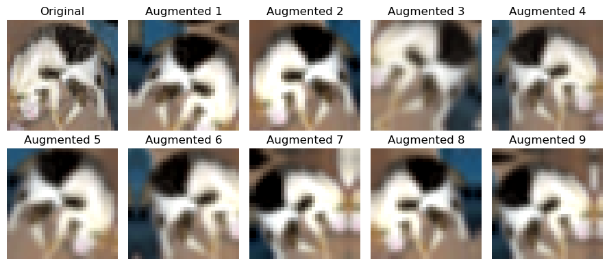
관찰: 같은 이미지여도 증식할 때마다 달라진다. 훈련에서는 training=True로 작동하지만, 검증·테스트에서는 증식을 끄고 변형하지 않은 이미지로 평가해야 한다.
def build_catdog_model(use_augmentation=False):
    inputs = keras.Input(shape=(32, 32, 3))
    x = inputs
    if use_augmentation:
        x = layers.RandomFlip("horizontal")(x)
        x = layers.RandomRotation(0.05)(x)
    x = layers.Rescaling(1.0 / 255)(x)
    x = layers.Conv2D(32, 3, padding="same", activation="relu")(x)
    x = layers.MaxPooling2D(2)(x)
    x = layers.Conv2D(64, 3, padding="same", activation="relu")(x)
    x = layers.MaxPooling2D(2)(x)
    x = layers.Conv2D(128, 3, padding="same", activation="relu")(x)
    x = layers.GlobalAveragePooling2D()(x)
    outputs = layers.Dense(1, activation="sigmoid")(x)
    model = keras.Model(inputs, outputs)
    model.compile(optimizer="adam", loss="binary_crossentropy", metrics=["accuracy"])
    return model

baseline_catdog = build_catdog_model(use_augmentation=False)
augmented_catdog = build_catdog_model(use_augmentation=True)

history_baseline = baseline_catdog.fit(
    catdog_x_train, catdog_y_train,
    validation_data=(catdog_x_val, catdog_y_val),
    epochs=5, batch_size=64, verbose=1,
    callbacks=[keras.callbacks.EarlyStopping(monitor="val_loss", patience=2, restore_best_weights=True)],
)
history_augmented = augmented_catdog.fit(
    catdog_x_train, catdog_y_train,
    validation_data=(catdog_x_val, catdog_y_val),
    epochs=5, batch_size=64, verbose=1,
    callbacks=[keras.callbacks.EarlyStopping(monitor="val_loss", patience=2, restore_best_weights=True)],
)
Epoch 1/5
32/32 ━━━━━━━━━━━━━━━━━━━━ 4s 38ms/step - accuracy: 0.4915 - loss: 0.6959 - val_accuracy: 0.5000 - val_loss: 0.6932
Epoch 2/5
32/32 ━━━━━━━━━━━━━━━━━━━━ 0s 4ms/step - accuracy: 0.5055 - loss: 0.6933 - val_accuracy: 0.5100 - val_loss: 0.6927
Epoch 3/5
32/32 ━━━━━━━━━━━━━━━━━━━━ 0s 4ms/step - accuracy: 0.5150 - loss: 0.6931 - val_accuracy: 0.5000 - val_loss: 0.6924
Epoch 4/5
32/32 ━━━━━━━━━━━━━━━━━━━━ 0s 4ms/step - accuracy: 0.5275 - loss: 0.6909 - val_accuracy: 0.5000 - val_loss: 0.7041
Epoch 5/5
32/32 ━━━━━━━━━━━━━━━━━━━━ 0s 4ms/step - accuracy: 0.5350 - loss: 0.6937 - val_accuracy: 0.5040 - val_loss: 0.6901
Epoch 1/5
32/32 ━━━━━━━━━━━━━━━━━━━━ 1s 11ms/step - accuracy: 0.5070 - loss: 0.6940 - val_accuracy: 0.5000 - val_loss: 0.6933
Epoch 2/5
32/32 ━━━━━━━━━━━━━━━━━━━━ 0s 8ms/step - accuracy: 0.5105 - loss: 0.6930 - val_accuracy: 0.5980 - val_loss: 0.6915
Epoch 3/5
32/32 ━━━━━━━━━━━━━━━━━━━━ 0s 8ms/step - accuracy: 0.5250 - loss: 0.6929 - val_accuracy: 0.5200 - val_loss: 0.6903
Epoch 4/5
32/32 ━━━━━━━━━━━━━━━━━━━━ 0s 8ms/step - accuracy: 0.5310 - loss: 0.6898 - val_accuracy: 0.5000 - val_loss: 0.7017
Epoch 5/5
32/32 ━━━━━━━━━━━━━━━━━━━━ 0s 8ms/step - accuracy: 0.5505 - loss: 0.6912 - val_accuracy: 0.5680 - val_loss: 0.6832
10.3.2비교는 검증 데이터로
두 모델 모두 같은 훈련·검증 데이터를 사용해야 한다. 데이터 증식이 항상 성능을 높이는 것은 아니므로 검증 손실과 검증 정확도를 보고 판단한다. 조기 종료 콜백의 restore_best_weights=True는 검증 손실이 가장 좋았던 가중치를 복원한다. 테스트셋은 아직 사용하지 않는다.
plt.figure(figsize=(7, 4))
for label, h in [("Baseline CNN", history_baseline), ("Augmented CNN", history_augmented)]:
    epochs = range(1, len(h.history["val_loss"]) + 1)
    plt.plot(epochs, h.history["val_loss"], label=label)
plt.xlabel("epoch")
plt.xticks(range(1, 6))
plt.ylabel("Validation loss")
plt.legend()
plt.tight_layout()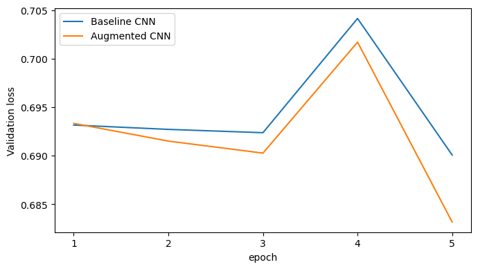
10.4전이 학습과 미세 조정: 사전훈련 CNN 재사용하기
10.4.1전이 학습: 이미 훈련된 CNN 재활용
ImageNet으로 사전훈련된 Xception의 합성곱 기저를 재사용하여 전이 학습을 실습한다. Xception은 채널 분리 합성곱·배치 정규화·잔차 연결을 조합한 CNN으로, 마지막 절에서 구조를 살펴본다.
weights="imagenet": 사전훈련 가중치 사용include_top=False: ImageNet 분류 출력층 제외transfer_base.trainable=False: 사전훈련 기저 동결새로운 이진 분류층을 추가하여 고양이·개를 분류함
입력 처리: Xception의 기본 입력 크기는 299×299이지만 분류층을 제외하면 96×96도 사용할 수 있다. 여기서는 32×32 CIFAR-10 이미지를 96×96으로 확대하고 픽셀값을 [-1, 1] 범위로 조정한다. 확대한다고 원본 이미지에 없던 세부 정보가 새로 생기는 것은 아니다.
실행 참고: Xception은 모델이 크므로 CPU에서는 훈련 시간이 길 수 있다. 사전훈련 가중치를 처음 사용할 때는 다운로드가 필요하며, 다운로드할 수 없다면 이 부분을 건너뛰고 다음 컴퓨터 비전 실습을 계속한다.
transfer_base = keras.applications.Xception(
    input_shape=(96, 96, 3), include_top=False, weights="imagenet"
)
transfer_base.trainable = False

inputs = keras.Input(shape=(32, 32, 3))
x = layers.RandomFlip("horizontal")(inputs)
x = layers.Resizing(96, 96)(x)
x = layers.Rescaling(1 / 127.5, offset=-1)(x)  # Xception 입력 범위 [-1, 1]
x = transfer_base(x, training=False)  # 미세 조정 중에도 BatchNorm은 추론 모드
x = layers.GlobalAveragePooling2D()(x)
outputs = layers.Dense(1, activation="sigmoid")(x)
transfer_model = keras.Model(inputs, outputs, name="catdog_xception_transfer")
transfer_model.compile(
    optimizer=keras.optimizers.Adam(learning_rate=1e-3),
    loss="binary_crossentropy", metrics=["accuracy"],
)
transfer_history = transfer_model.fit(
    catdog_x_train, catdog_y_train,
    validation_data=(catdog_x_val, catdog_y_val),
    epochs=4, batch_size=16, verbose=1,
    callbacks=[keras.callbacks.EarlyStopping(monitor="val_loss", patience=2, restore_best_weights=True)],
)
Downloading data from https://storage.googleapis.com/tensorflow/keras-applications/xception/xception_weights_tf_dim_ordering_tf_kernels_notop.h5
83683744/83683744 ━━━━━━━━━━━━━━━━━━━━ 10s 0us/step
Epoch 1/4
2026-11-10 15:59:51.186580: E external/local_xla/xla/stream_executor/cuda/cuda_timer.cc:86] Delay kernel timed out: measured time has sub-optimal accuracy. There may be a missing warmup execution, please investigate in Nsight Systems.
2026-11-10 15:59:51.359380: E external/local_xla/xla/stream_executor/cuda/cuda_timer.cc:86] Delay kernel timed out: measured time has sub-optimal accuracy. There may be a missing warmup execution, please investigate in Nsight Systems.
2026-11-10 15:59:51.862379: E external/local_xla/xla/stream_executor/cuda/cuda_timer.cc:86] Delay kernel timed out: measured time has sub-optimal accuracy. There may be a missing warmup execution, please investigate in Nsight Systems.
2026-11-10 15:59:52.033179: E external/local_xla/xla/stream_executor/cuda/cuda_timer.cc:86] Delay kernel timed out: measured time has sub-optimal accuracy. There may be a missing warmup execution, please investigate in Nsight Systems.
2026-11-10 15:59:52.614399: E external/local_xla/xla/stream_executor/cuda/cuda_timer.cc:86] Delay kernel timed out: measured time has sub-optimal accuracy. There may be a missing warmup execution, please investigate in Nsight Systems.
2026-11-10 15:59:52.804008: E external/local_xla/xla/stream_executor/cuda/cuda_timer.cc:86] Delay kernel timed out: measured time has sub-optimal accuracy. There may be a missing warmup execution, please investigate in Nsight Systems.
2026-11-10 15:59:53.345483: E external/local_xla/xla/stream_executor/cuda/cuda_timer.cc:86] Delay kernel timed out: measured time has sub-optimal accuracy. There may be a missing warmup execution, please investigate in Nsight Systems.
2026-11-10 15:59:53.558186: E external/local_xla/xla/stream_executor/cuda/cuda_timer.cc:86] Delay kernel timed out: measured time has sub-optimal accuracy. There may be a missing warmup execution, please investigate in Nsight Systems.
121/125 ━━━━━━━━━━━━━━━━━━━━ 0s 5ms/step - accuracy: 0.6645 - loss: 0.57432026-11-10 16:00:00.144105: E external/local_xla/xla/stream_executor/cuda/cuda_timer.cc:86] Delay kernel timed out: measured time has sub-optimal accuracy. There may be a missing warmup execution, please investigate in Nsight Systems.
2026-11-10 16:00:00.321471: E external/local_xla/xla/stream_executor/cuda/cuda_timer.cc:86] Delay kernel timed out: measured time has sub-optimal accuracy. There may be a missing warmup execution, please investigate in Nsight Systems.
2026-11-10 16:00:00.867663: E external/local_xla/xla/stream_executor/cuda/cuda_timer.cc:86] Delay kernel timed out: measured time has sub-optimal accuracy. There may be a missing warmup execution, please investigate in Nsight Systems.
2026-11-10 16:00:01.052798: E external/local_xla/xla/stream_executor/cuda/cuda_timer.cc:86] Delay kernel timed out: measured time has sub-optimal accuracy. There may be a missing warmup execution, please investigate in Nsight Systems.
2026-11-10 16:00:01.664193: E external/local_xla/xla/stream_executor/cuda/cuda_timer.cc:86] Delay kernel timed out: measured time has sub-optimal accuracy. There may be a missing warmup execution, please investigate in Nsight Systems.
2026-11-10 16:00:01.859779: E external/local_xla/xla/stream_executor/cuda/cuda_timer.cc:86] Delay kernel timed out: measured time has sub-optimal accuracy. There may be a missing warmup execution, please investigate in Nsight Systems.
2026-11-10 16:00:02.446436: E external/local_xla/xla/stream_executor/cuda/cuda_timer.cc:86] Delay kernel timed out: measured time has sub-optimal accuracy. There may be a missing warmup execution, please investigate in Nsight Systems.
2026-11-10 16:00:02.663420: E external/local_xla/xla/stream_executor/cuda/cuda_timer.cc:86] Delay kernel timed out: measured time has sub-optimal accuracy. There may be a missing warmup execution, please investigate in Nsight Systems.
2026-11-10 16:00:02.890899: E external/local_xla/xla/stream_executor/cuda/cuda_timer.cc:86] Delay kernel timed out: measured time has sub-optimal accuracy. There may be a missing warmup execution, please investigate in Nsight Systems.
2026-11-10 16:00:03.106796: E external/local_xla/xla/stream_executor/cuda/cuda_timer.cc:86] Delay kernel timed out: measured time has sub-optimal accuracy. There may be a missing warmup execution, please investigate in Nsight Systems.
125/125 ━━━━━━━━━━━━━━━━━━━━ 19s 89ms/step - accuracy: 0.7410 - loss: 0.4968 - val_accuracy: 0.7760 - val_loss: 0.4607
Epoch 2/4
125/125 ━━━━━━━━━━━━━━━━━━━━ 1s 7ms/step - accuracy: 0.7975 - loss: 0.4116 - val_accuracy: 0.7960 - val_loss: 0.4376
Epoch 3/4
125/125 ━━━━━━━━━━━━━━━━━━━━ 1s 7ms/step - accuracy: 0.8290 - loss: 0.3715 - val_accuracy: 0.7800 - val_loss: 0.4577
Epoch 4/4
125/125 ━━━━━━━━━━━━━━━━━━━━ 1s 7ms/step - accuracy: 0.8325 - loss: 0.3582 - val_accuracy: 0.7620 - val_loss: 0.4803
판단: 사전훈련 모델이 좋은 결과를 보장하지는 않는다. 사전훈련 데이터와 목표 데이터가 얼마나 비슷한지, 입력 이미지의 해상도, 사용하는 데이터의 양, 전처리 방식이 결과에 영향을 준다.
10.4.2미세 조정(fine-tuning)은 언제 필요한가?
특성 추출 단계에서는 Xception 기저를 동결하고 새로운 분류층만 훈련한다. 미세 조정에서는 Xception의 마지막 일부 층만 동결 해제하고 작은 학습률로 추가 훈련할 수 있다. 훈련 가능한 층을 바꾼 뒤에는 다시 compile()해야 한다.
Xception에는 BatchNormalization 층이 많이 포함되어 있다. 미세 조정 시 배치 통계가 크게 바뀌지 않도록 이 층은 동결하고, 앞에서 사용한 transfer_base(x, training=False) 호출도 유지한다.
transfer_base.trainable = True
for layer in transfer_base.layers[:-20]:
    layer.trainable = False
for layer in transfer_base.layers:
    if isinstance(layer, layers.BatchNormalization):
        layer.trainable = False

print("미세 조정 대상 가중치 수:", len(transfer_base.trainable_weights))
transfer_model.compile(
    optimizer=keras.optimizers.Adam(learning_rate=1e-5),
    loss="binary_crossentropy", metrics=["accuracy"],
)
transfer_history = transfer_model.fit(
    catdog_x_train, catdog_y_train,
    validation_data=(catdog_x_val, catdog_y_val),
    epochs=2, batch_size=16, verbose=1,
    callbacks=[keras.callbacks.EarlyStopping(monitor="val_loss", patience=1, restore_best_weights=True)],
)
미세 조정 대상 가중치 수: 11
Epoch 1/2
2026-11-10 16:00:11.766868: E external/local_xla/xla/stream_executor/cuda/cuda_timer.cc:86] Delay kernel timed out: measured time has sub-optimal accuracy. There may be a missing warmup execution, please investigate in Nsight Systems.
2026-11-10 16:00:11.935435: E external/local_xla/xla/stream_executor/cuda/cuda_timer.cc:86] Delay kernel timed out: measured time has sub-optimal accuracy. There may be a missing warmup execution, please investigate in Nsight Systems.
2026-11-10 16:00:12.293479: E external/local_xla/xla/stream_executor/cuda/cuda_timer.cc:86] Delay kernel timed out: measured time has sub-optimal accuracy. There may be a missing warmup execution, please investigate in Nsight Systems.
2026-11-10 16:00:12.477266: E external/local_xla/xla/stream_executor/cuda/cuda_timer.cc:86] Delay kernel timed out: measured time has sub-optimal accuracy. There may be a missing warmup execution, please investigate in Nsight Systems.
125/125 ━━━━━━━━━━━━━━━━━━━━ 10s 33ms/step - accuracy: 0.8250 - loss: 0.3619 - val_accuracy: 0.8040 - val_loss: 0.4254
Epoch 2/2
125/125 ━━━━━━━━━━━━━━━━━━━━ 1s 10ms/step - accuracy: 0.8610 - loss: 0.3148 - val_accuracy: 0.8140 - val_loss: 0.4157
10.4.3마지막으로 테스트 데이터에서 평가
검증 데이터에서 선택한 모델만 테스트한다. 서로 다른 접근법의 성능을 비교할 때 같은 검증셋과 같은 평가 기준을 사용한다.
candidates = {
    "기준 CNN": (baseline_catdog, history_baseline),
    "증식 CNN": (augmented_catdog, history_augmented),
}
if transfer_history is not None:
    candidates["전이 학습"] = (transfer_model, transfer_history)

for name, (_, h) in candidates.items():
    print(name, "최소 검증 손실:", round(min(h.history["val_loss"]), 4),
          "최종 검증 정확도:", round(h.history["val_accuracy"][-1], 4))

best_name = min(candidates, key=lambda key: min(candidates[key][1].history["val_loss"]))
best_model = candidates[best_name][0]
print("검증 손실로 선택한 모델:", best_name)

catdog_test_loss, catdog_test_acc = best_model.evaluate(
    catdog_x_test, catdog_y_test, verbose=0
)
print(f"선택 모델의 테스트 정확도: {catdog_test_acc:.3f}")
기준 CNN 최소 검증 손실: 0.6856 최종 검증 정확도: 0.568
증식 CNN 최소 검증 손실: 0.6923 최종 검증 정확도: 0.5
전이 학습 최소 검증 손실: 0.4157 최종 검증 정확도: 0.814
검증 손실로 선택한 모델: 전이 학습
2026-11-10 16:00:22.895322: E external/local_xla/xla/service/slow_operation_alarm.cc:73] Trying algorithm eng3{k11=2} for conv (f32[32,256,12,12]{3,2,1,0}, u8[0]{0}) custom-call(f32[32,256,12,12]{3,2,1,0}, f32[256,1,3,3]{3,2,1,0}), window={size=3x3 pad=1_1x1_1}, dim_labels=bf01_oi01->bf01, feature_group_count=256, custom_call_target="__cudnn$convForward", backend_config={"operation_queue_id":"0","wait_on_operation_queues":[],"cudnn_conv_backend_config":{"activation_mode":"kNone","conv_result_scale":1,"side_input_scale":0,"leakyrelu_alpha":0},"force_earliest_schedule":false,"reification_cost":[]} is taking a while...
2026-11-10 16:00:24.873025: E external/local_xla/xla/service/slow_operation_alarm.cc:140] The operation took 2.977789763s
Trying algorithm eng3{k11=2} for conv (f32[32,256,12,12]{3,2,1,0}, u8[0]{0}) custom-call(f32[32,256,12,12]{3,2,1,0}, f32[256,1,3,3]{3,2,1,0}), window={size=3x3 pad=1_1x1_1}, dim_labels=bf01_oi01->bf01, feature_group_count=256, custom_call_target="__cudnn$convForward", backend_config={"operation_queue_id":"0","wait_on_operation_queues":[],"cudnn_conv_backend_config":{"activation_mode":"kNone","conv_result_scale":1,"side_input_scale":0,"leakyrelu_alpha":0},"force_earliest_schedule":false,"reification_cost":[]} is taking a while...
2026-11-10 16:00:25.951636: E external/local_xla/xla/service/slow_operation_alarm.cc:73] Trying algorithm eng48{k2=2,k6=0,k13=2,k14=0,k22=2} for conv (f32[32,728,12,12]{3,2,1,0}, u8[0]{0}) custom-call(f32[32,256,12,12]{3,2,1,0}, f32[728,256,1,1]{3,2,1,0}), window={size=1x1}, dim_labels=bf01_oi01->bf01, custom_call_target="__cudnn$convForward", backend_config={"operation_queue_id":"0","wait_on_operation_queues":[],"cudnn_conv_backend_config":{"activation_mode":"kNone","conv_result_scale":1,"side_input_scale":0,"leakyrelu_alpha":0},"force_earliest_schedule":false,"reification_cost":[]} is taking a while...
2026-11-10 16:00:26.444698: E external/local_xla/xla/service/slow_operation_alarm.cc:140] The operation took 1.49313084s
Trying algorithm eng48{k2=2,k6=0,k13=2,k14=0,k22=2} for conv (f32[32,728,12,12]{3,2,1,0}, u8[0]{0}) custom-call(f32[32,256,12,12]{3,2,1,0}, f32[728,256,1,1]{3,2,1,0}), window={size=1x1}, dim_labels=bf01_oi01->bf01, custom_call_target="__cudnn$convForward", backend_config={"operation_queue_id":"0","wait_on_operation_queues":[],"cudnn_conv_backend_config":{"activation_mode":"kNone","conv_result_scale":1,"side_input_scale":0,"leakyrelu_alpha":0},"force_earliest_schedule":false,"reification_cost":[]} is taking a while...
2026-11-10 16:00:27.001351: E external/local_xla/xla/stream_executor/cuda/cuda_timer.cc:86] Delay kernel timed out: measured time has sub-optimal accuracy. There may be a missing warmup execution, please investigate in Nsight Systems.
2026-11-10 16:00:27.239405: E external/local_xla/xla/stream_executor/cuda/cuda_timer.cc:86] Delay kernel timed out: measured time has sub-optimal accuracy. There may be a missing warmup execution, please investigate in Nsight Systems.
2026-11-10 16:00:27.864737: E external/local_xla/xla/stream_executor/cuda/cuda_timer.cc:86] Delay kernel timed out: measured time has sub-optimal accuracy. There may be a missing warmup execution, please investigate in Nsight Systems.
2026-11-10 16:00:28.054893: E external/local_xla/xla/stream_executor/cuda/cuda_timer.cc:86] Delay kernel timed out: measured time has sub-optimal accuracy. There may be a missing warmup execution, please investigate in Nsight Systems.
2026-11-10 16:00:28.204184: E external/local_xla/xla/stream_executor/cuda/cuda_timer.cc:86] Delay kernel timed out: measured time has sub-optimal accuracy. There may be a missing warmup execution, please investigate in Nsight Systems.
2026-11-10 16:00:28.539366: E external/local_xla/xla/stream_executor/cuda/cuda_timer.cc:86] Delay kernel timed out: measured time has sub-optimal accuracy. There may be a missing warmup execution, please investigate in Nsight Systems.
2026-11-10 16:00:28.664664: E external/local_xla/xla/service/slow_operation_alarm.cc:73] Trying algorithm eng3{k11=2} for conv (f32[32,728,6,6]{3,2,1,0}, u8[0]{0}) custom-call(f32[32,728,6,6]{3,2,1,0}, f32[728,1,3,3]{3,2,1,0}), window={size=3x3 pad=1_1x1_1}, dim_labels=bf01_oi01->bf01, feature_group_count=728, custom_call_target="__cudnn$convForward", backend_config={"operation_queue_id":"0","wait_on_operation_queues":[],"cudnn_conv_backend_config":{"activation_mode":"kNone","conv_result_scale":1,"side_input_scale":0,"leakyrelu_alpha":0},"force_earliest_schedule":false,"reification_cost":[]} is taking a while...
2026-11-10 16:00:28.813913: E external/local_xla/xla/stream_executor/cuda/cuda_timer.cc:86] Delay kernel timed out: measured time has sub-optimal accuracy. There may be a missing warmup execution, please investigate in Nsight Systems.
2026-11-10 16:00:28.817794: E external/local_xla/xla/service/slow_operation_alarm.cc:140] The operation took 1.153287012s
Trying algorithm eng3{k11=2} for conv (f32[32,728,6,6]{3,2,1,0}, u8[0]{0}) custom-call(f32[32,728,6,6]{3,2,1,0}, f32[728,1,3,3]{3,2,1,0}), window={size=3x3 pad=1_1x1_1}, dim_labels=bf01_oi01->bf01, feature_group_count=728, custom_call_target="__cudnn$convForward", backend_config={"operation_queue_id":"0","wait_on_operation_queues":[],"cudnn_conv_backend_config":{"activation_mode":"kNone","conv_result_scale":1,"side_input_scale":0,"leakyrelu_alpha":0},"force_earliest_schedule":false,"reification_cost":[]} is taking a while...
2026-11-10 16:00:29.402672: E external/local_xla/xla/stream_executor/cuda/cuda_timer.cc:86] Delay kernel timed out: measured time has sub-optimal accuracy. There may be a missing warmup execution, please investigate in Nsight Systems.
2026-11-10 16:00:29.589877: E external/local_xla/xla/stream_executor/cuda/cuda_timer.cc:86] Delay kernel timed out: measured time has sub-optimal accuracy. There may be a missing warmup execution, please investigate in Nsight Systems.
2026-11-10 16:00:30.132537: E external/local_xla/xla/stream_executor/cuda/cuda_timer.cc:86] Delay kernel timed out: measured time has sub-optimal accuracy. There may be a missing warmup execution, please investigate in Nsight Systems.
2026-11-10 16:00:30.336955: E external/local_xla/xla/stream_executor/cuda/cuda_timer.cc:86] Delay kernel timed out: measured time has sub-optimal accuracy. There may be a missing warmup execution, please investigate in Nsight Systems.
2026-11-10 16:00:34.195667: E external/local_xla/xla/stream_executor/cuda/cuda_timer.cc:86] Delay kernel timed out: measured time has sub-optimal accuracy. There may be a missing warmup execution, please investigate in Nsight Systems.
2026-11-10 16:00:34.381763: E external/local_xla/xla/stream_executor/cuda/cuda_timer.cc:86] Delay kernel timed out: measured time has sub-optimal accuracy. There may be a missing warmup execution, please investigate in Nsight Systems.
2026-11-10 16:00:34.931636: E external/local_xla/xla/stream_executor/cuda/cuda_timer.cc:86] Delay kernel timed out: measured time has sub-optimal accuracy. There may be a missing warmup execution, please investigate in Nsight Systems.
2026-11-10 16:00:35.115967: E external/local_xla/xla/stream_executor/cuda/cuda_timer.cc:86] Delay kernel timed out: measured time has sub-optimal accuracy. There may be a missing warmup execution, please investigate in Nsight Systems.
2026-11-10 16:00:35.730353: E external/local_xla/xla/stream_executor/cuda/cuda_timer.cc:86] Delay kernel timed out: measured time has sub-optimal accuracy. There may be a missing warmup execution, please investigate in Nsight Systems.
2026-11-10 16:00:35.928421: E external/local_xla/xla/stream_executor/cuda/cuda_timer.cc:86] Delay kernel timed out: measured time has sub-optimal accuracy. There may be a missing warmup execution, please investigate in Nsight Systems.
2026-11-10 16:00:36.506118: E external/local_xla/xla/stream_executor/cuda/cuda_timer.cc:86] Delay kernel timed out: measured time has sub-optimal accuracy. There may be a missing warmup execution, please investigate in Nsight Systems.
2026-11-10 16:00:36.725193: E external/local_xla/xla/stream_executor/cuda/cuda_timer.cc:86] Delay kernel timed out: measured time has sub-optimal accuracy. There may be a missing warmup execution, please investigate in Nsight Systems.
2026-11-10 16:00:36.947724: E external/local_xla/xla/stream_executor/cuda/cuda_timer.cc:86] Delay kernel timed out: measured time has sub-optimal accuracy. There may be a missing warmup execution, please investigate in Nsight Systems.
선택 모델의 테스트 정확도: 0.822
해석: 어떤 모델이 선택되었는가? 데이터 증식이 검증 손실을 줄였는가? 전이 학습의 효과가 불분명하다면 가능한 이유를 두 가지 생각해보자.
10.5CNN 아키텍처의 세 가지 개선 아이디어
잔차 연결, 배치 정규화, 채널 분리 합성곱은 CNN 구조를 개선할 때 활용하는 방법이다. 큰 네트워크를 새로 훈련하기보다 각 코드가 어떤 문제를 해결하는지 확인한다.
10.5.1잔차 연결: 입력을 출력에 더하기
잔차 연결(residual connection)은 블록을 통과한 값에 블록의 입력을 더한다. 더할 텐서의 모양이 같아야 한다. 모양이 다르면 1×1 합성곱 등으로 맞춘다.
res_inputs = keras.Input(shape=(32, 32, 3))
x = layers.Conv2D(16, 3, padding="same", activation="relu")(res_inputs)
skip = x  # 블록 입력 저장
x = layers.Conv2D(16, 3, padding="same")(x)
x = layers.Add()([x, skip])
x = layers.Activation("relu")(x)
res_model = keras.Model(res_inputs, x)
print("입력:", res_model.input_shape, "출력:", res_model.output_shape)
입력: (None, 32, 32, 3) 출력: (None, 32, 32, 16)
확인: 만약 두 번째 합성곱 층의 필터 수가 32라면 skip의 채널 16과 달라져 그대로는 더할 수 없다. 이때 Conv2D(32, 1) 같은 층으로 skip의 채널 수를 맞출 수 있다.
10.5.2배치 정규화: 중간 출력의 크기 조정
배치 정규화(batch normalization)는 층의 중간 출력에 정규화를 적용한다. 훈련과 평가 모드의 동작이 다르므로 전이 학습에서 동결 여부에 주의해야 한다.
bn_inputs = keras.Input(shape=(32, 32, 3))
x = layers.Conv2D(16, 3, padding="same", use_bias=False)(bn_inputs)
x = layers.BatchNormalization()(x)
x = layers.Activation("relu")(x)
bn_model = keras.Model(bn_inputs, x)
print("출력 모양:", bn_model.output_shape)
출력 모양: (None, 32, 32, 16)
10.5.3채널 분리 합성곱: 적은 파라미터로 처리하기
SeparableConv2D는 채널별 합성곱(depthwise)과 1×1 합성곱(pointwise)을 결합한다. 일반 Conv2D와 비교해 학습할 가중치 수를 줄일 수 있다. 연산량이 적다는 사실만으로 모든 하드웨어에서 항상 더 빠르다고 보장할 수는 없다.
comparison_input = keras.Input(shape=(32, 32, 3))
normal_conv = layers.Conv2D(64, 3, use_bias=False)
separable_conv = layers.SeparableConv2D(64, 3, use_bias=False)
normal_conv(comparison_input)
separable_conv(comparison_input)

print("Conv2D 가중치 수:", normal_conv.count_params())
print("SeparableConv2D 가중치 수:", separable_conv.count_params())
Conv2D 가중치 수: 1728
SeparableConv2D 가중치 수: 219
해석: 두 층의 출력 채널 수는 64로 같지만 파라미터 수는 다르다. 모델 설계에서는 정확도뿐 아니라 데이터 양·연산량·실행 시간도 함께 고려한다.
10.5.4Xception: 세 가지 개선 아이디어를 결합한 CNN
Xception은 잔차 연결, 배치 정규화, 채널 분리 합성곱을 하나의 아키텍처에 함께 사용한다. 큰 구조는 세 부분으로 나눠 볼 수 있다.
| 부분 | 주요 역할 |
|---|---|
| Entry Flow | 일반 합성곱으로 초기 특성을 추출한 후 채널 분리 합성곱과 풀링으로 공간 크기를 줄인다. |
| Middle Flow | 채널 분리 합성곱과 잔차 연결이 있는 블록을 8회 반복해 특성을 가공한다. |
| Exit Flow | 특성을 더 높은 수준으로 변환하고 최종 2048채널 특성맵을 만든다. |
중간 블록의 핵심 관계는 다음처럼 단순화할 수 있다. 실제 층에는 활성화 함수가 들어가고, 블록 종류에 따라 차원 조정이나 다운샘플링이 추가된다.
                     ┌──────── 잔차 연결 ────────┐
입력 x ───────────┤                           Add → 출력
└→ (SeparableConv2D → BN) × 3 ──┘SeparableConv2D: 공간 필터링과 채널 결합을 나누어 수행한다.BatchNormalization: 합성곱의 중간 출력을 정규화한다.Add: 변환된 특성에 블록 입력을 더하는 잔차 연결이다.
앞에서 사용한 include_top=False는 Xception의 ImageNet 분류층을 제외하고 특성 추출 부분만 가져온다는 뜻이다. 여기에 GlobalAveragePooling2D와 이진 분류 출력층을 연결하여 고양이·개 분류에 활용했다.
질문: 이 세 가지 기법의 역할이 서로 다른데도 하나의 블록에서 함께 쓰이는 이유는 무엇일까?
# 전이 학습에서 불러온 실제 Xception 층의 구성을 살펴본다.
if transfer_base is not None:
    for cls in (layers.SeparableConv2D, layers.BatchNormalization, layers.Add):
        count = sum(isinstance(layer, cls) for layer in transfer_base.layers)
        print(f"{cls.__name__}: {count}")
    print("Xception feature shape:", transfer_base.output_shape)
else:
    print("Xception 모델이 로드되지 않아 구조 확인을 건너뜁니다.")
SeparableConv2D: 34
BatchNormalization: 40
Add: 12
Xception feature shape: (None, 3, 3, 2048)
10.6Keras와 PyTorch에서 같은 개념 찾기
| 개념 | Keras | PyTorch |
|---|---|---|
| 2차원 합성곱 | layers.Conv2D | nn.Conv2d |
| 맥스 풀링 | layers.MaxPooling2D | nn.MaxPool2d |
| 전역 평균 풀링 | layers.GlobalAveragePooling2D | nn.AdaptiveAvgPool2d(1) 후 펼치기 |
| 배치 정규화 | layers.BatchNormalization | nn.BatchNorm2d |
| 채널 분리 합성곱 | layers.SeparableConv2D | depthwise nn.Conv2d(groups=입력채널) + pointwise nn.Conv2d(1) |
| 잔차 연결 | layers.Add() | x + skip |
| 사전훈련 모델 재사용 | keras.applications | torchvision.models |
주의: PyTorch 합성곱의 이미지 입력은 NCHW, Keras의 기본 이미지 입력은 NHWC다. 마지막 분류층의 PyTorch CrossEntropyLoss는 logits를 기대한다.
10.7PyTorch 실습: 단순화한 Xception으로 이미지 분류하기
세 가지 CNN 개선 기법을 하나의 모델에 결합한다. 채널 분리 합성곱은 연산을 나누어 수행하고, 배치 정규화는 중간 출력을 정규화하며, 잔차 연결은 블록 입력을 출력에 더한다.
여기서는 Xception의 핵심 설계 아이디어만 가져온 작은 모델을 직접 구현한다. 실제 Xception의 Entry·Middle·Exit Flow와 층 구성, 사전훈련 가중치를 그대로 재현한 모델은 아니다. 위에서 사용한 ImageNet 사전훈련 Xception과 달리 처음부터 훈련한다.
질문: 세 가지 기법을 하나의 잔차 블록으로 구현하려면 forward()에서 무엇을 더해야 할까?
10.7.1채널 분리 합성곱과 잔차 블록 구현
groups=in_channels인3×3 Conv2d는 채널마다 별도의 공간 필터를 적용한다(Depthwise).1×1 Conv2d는 채널을 결합해 출력 채널을 만든다(Pointwise).두 경로의 출력 모양이 다르면
1×1 Conv2d로 잔차 경로의 채널·공간 크기를 맞춘다.
아래 잔차 블록은 학습 가능한 두 개의 채널 분리 합성곱과 배치 정규화를 포함한다.
class DepthwiseSeparableConv(nn.Module):
    def __init__(self, in_channels, out_channels):
        super().__init__()
        self.depthwise = nn.Conv2d(
            in_channels, in_channels, kernel_size=3, padding=1,
            groups=in_channels, bias=False
        )
        self.pointwise = nn.Conv2d(in_channels, out_channels, kernel_size=1, bias=False)

    def forward(self, x):
        x = self.depthwise(x)
        return self.pointwise(x)


class MiniXceptionBlock(nn.Module):
    def __init__(self, in_channels, out_channels, stride=1):
        super().__init__()
        self.main = nn.Sequential(
            nn.ReLU(),
            DepthwiseSeparableConv(in_channels, out_channels),
            nn.BatchNorm2d(out_channels),
            nn.ReLU(),
            DepthwiseSeparableConv(out_channels, out_channels),
            nn.BatchNorm2d(out_channels),
            nn.MaxPool2d(kernel_size=3, stride=2, padding=1) if stride == 2 else nn.Identity(),
        )
        self.skip = (
            nn.Identity() if stride == 1 and in_channels == out_channels else
            nn.Sequential(
                nn.Conv2d(in_channels, out_channels, kernel_size=1, stride=stride, bias=False),
                nn.BatchNorm2d(out_channels),
            )
        )

    def forward(self, x):
        return self.main(x) + self.skip(x)


class MiniXception(nn.Module):
    def __init__(self):
        super().__init__()
        self.stem = nn.Sequential(
            nn.Conv2d(3, 24, kernel_size=3, padding=1, bias=False),
            nn.BatchNorm2d(24),
            nn.ReLU(),
        )
        self.entry = MiniXceptionBlock(24, 32, stride=2)
        self.middle = MiniXceptionBlock(32, 32)
        self.exit = MiniXceptionBlock(32, 64, stride=2)
        self.pool = nn.AdaptiveAvgPool2d(1)
        self.classifier = nn.Linear(64, 1)

    def forward(self, x):
        x = self.stem(x)
        x = self.entry(x)
        x = self.middle(x)
        x = self.exit(x)
        x = self.pool(x).flatten(1)
        return self.classifier(x).squeeze(1)  # logits: (batch,)


torch.manual_seed(42)
mini_xception = MiniXception().to(device)

with torch.no_grad():
    demo_logits = mini_xception.eval()(torch.zeros(2, 3, 32, 32, device=device))
print('Model output shape:', tuple(demo_logits.shape))
print('Trainable parameters:', sum(p.numel() for p in mini_xception.parameters() if p.requires_grad))
Model output shape: (2,)
Trainable parameters: 16209
관찰: 입력은 (배치, 3, 32, 32)이고, 출력은 이미지마다 하나의 logit이다. 이진 분류이므로 BCEWithLogitsLoss를 사용할 수 있다. Sigmoid는 손실 함수 내부에서 처리하므로 모델의 forward()에 넣지 않는다.
채널 분리 합성곱이 일반 합성곱보다 적은 가중치를 사용한다는 점을 확인해보자.
regular = nn.Conv2d(32, 64, kernel_size=3, padding=1, bias=False)
separable = DepthwiseSeparableConv(32, 64)
print('Regular Conv2d parameters:', sum(p.numel() for p in regular.parameters()))
print('Depthwise separable parameters:', sum(p.numel() for p in separable.parameters()))
Regular Conv2d parameters: 18432
Depthwise separable parameters: 2336
10.7.2CIFAR-10 고양이·개 이미지에 적용하기
이진 분류에 사용한 고양이·개 이미지를 PyTorch 입력 형식인 NCHW로 변환한다. 픽셀값은 [0, 1]로 조정한다. 훈련과 검증에는 각각 별도의 DataLoader를 사용한다.
사전훈련 가중치를 사용하지 않으므로 이 모델의 검증 정확도가 앞서 사용한 Xception 전이 학습보다 높을 것이라고 기대할 이유는 없다.
mini_x_train = torch.from_numpy(catdog_x_train / 255.0).permute(0, 3, 1, 2).contiguous()
mini_y_train = torch.from_numpy(catdog_y_train)
mini_x_val = torch.from_numpy(catdog_x_val / 255.0).permute(0, 3, 1, 2).contiguous()
mini_y_val = torch.from_numpy(catdog_y_val)

mini_train_loader = DataLoader(
    TensorDataset(mini_x_train, mini_y_train), batch_size=32, shuffle=True
)
mini_val_loader = DataLoader(
    TensorDataset(mini_x_val, mini_y_val), batch_size=64, shuffle=False
)

mini_loss_fn = nn.BCEWithLogitsLoss()
mini_optimizer = torch.optim.Adam(mini_xception.parameters(), lr=1e-3)


def run_mini_epoch(model, loader, optimizer=None):
    training = optimizer is not None
    model.train(training)
    total_loss, correct, n = 0.0, 0, 0
    with torch.set_grad_enabled(training):
        for xb, yb in loader:
            xb, yb = xb.to(device), yb.to(device)
            if training:
                optimizer.zero_grad()
            logits = model(xb)
            loss = mini_loss_fn(logits, yb)
            if training:
                loss.backward()
                optimizer.step()
            total_loss += loss.item() * len(yb)
            correct += ((logits >= 0).float() == yb).sum().item()
            n += len(yb)
    return total_loss / n, correct / n


mini_history = {'loss': [], 'val_loss': [], 'accuracy': [], 'val_accuracy': []}
for epoch in range(20):
    train_loss, train_acc = run_mini_epoch(mini_xception, mini_train_loader, mini_optimizer)
    val_loss, val_acc = run_mini_epoch(mini_xception, mini_val_loader)
    mini_history['loss'].append(train_loss)
    mini_history['val_loss'].append(val_loss)
    mini_history['accuracy'].append(train_acc)
    mini_history['val_accuracy'].append(val_acc)
    print(f'Epoch {epoch + 1}: loss={train_loss:.3f}, accuracy={train_acc:.3f}, '
          f'val_loss={val_loss:.3f}, val_accuracy={val_acc:.3f}')
Epoch 1: loss=0.690, accuracy=0.545, val_loss=0.671, val_accuracy=0.594
Epoch 2: loss=0.654, accuracy=0.626, val_loss=0.654, val_accuracy=0.624
Epoch 3: loss=0.634, accuracy=0.652, val_loss=0.648, val_accuracy=0.634
Epoch 4: loss=0.601, accuracy=0.684, val_loss=0.624, val_accuracy=0.650
Epoch 5: loss=0.578, accuracy=0.699, val_loss=0.645, val_accuracy=0.672
Epoch 6: loss=0.551, accuracy=0.720, val_loss=0.624, val_accuracy=0.674
Epoch 7: loss=0.518, accuracy=0.757, val_loss=0.706, val_accuracy=0.596
Epoch 8: loss=0.505, accuracy=0.764, val_loss=0.670, val_accuracy=0.648
Epoch 9: loss=0.470, accuracy=0.787, val_loss=0.803, val_accuracy=0.590
Epoch 10: loss=0.444, accuracy=0.790, val_loss=0.757, val_accuracy=0.658
Epoch 11: loss=0.416, accuracy=0.809, val_loss=0.655, val_accuracy=0.662
Epoch 12: loss=0.365, accuracy=0.836, val_loss=0.837, val_accuracy=0.634
Epoch 13: loss=0.363, accuracy=0.840, val_loss=0.638, val_accuracy=0.674
Epoch 14: loss=0.332, accuracy=0.852, val_loss=0.670, val_accuracy=0.690
Epoch 15: loss=0.289, accuracy=0.883, val_loss=0.716, val_accuracy=0.682
Epoch 16: loss=0.267, accuracy=0.891, val_loss=0.673, val_accuracy=0.702
Epoch 17: loss=0.254, accuracy=0.903, val_loss=0.776, val_accuracy=0.680
Epoch 18: loss=0.222, accuracy=0.916, val_loss=0.862, val_accuracy=0.648
Epoch 19: loss=0.183, accuracy=0.936, val_loss=0.959, val_accuracy=0.694
Epoch 20: loss=0.197, accuracy=0.924, val_loss=0.745, val_accuracy=0.706
10.7.3학습 곡선과 예측 결과 확인
훈련과 검증의 손실 및 정확도를 비교하고, 검증 이미지에서 예측 결과를 관찰한다. 모델의 출력 logit에 sigmoid()를 적용하면 개(dog)일 예측 점수를 0과 1 사이의 값으로 나타낼 수 있다.
fig, axes = plt.subplots(1, 2, figsize=(10, 3.5))
epochs = range(1, len(mini_history['loss']) + 1)

axes[0].plot(epochs, mini_history['loss'], marker='o', label='Train')
axes[0].plot(epochs, mini_history['val_loss'], marker='o', label='Validation')
axes[0].set(xlabel='Epoch', ylabel='Loss', title='Mini Xception: Loss')
axes[0].set_xticks(range(1, 21, 2))
axes[0].legend()

axes[1].plot(epochs, mini_history['accuracy'], marker='o', label='Train')
axes[1].plot(epochs, mini_history['val_accuracy'], marker='o', label='Validation')
axes[1].set(xlabel='Epoch', ylabel='Accuracy', title='Mini Xception: Accuracy')
axes[1].set_xticks(range(1, 21, 2))
axes[1].legend()

plt.tight_layout()

mini_x_examples = mini_x_val[:8].to(device)
mini_xception.eval()
with torch.no_grad():
    mini_dog_scores = torch.sigmoid(mini_xception(mini_x_examples)).cpu().numpy()

fig, axes = plt.subplots(2, 4, figsize=(10, 5))
for i, ax in enumerate(axes.flat):
    ax.imshow(catdog_x_val[i].astype('uint8'))
    true_label = 'dog' if catdog_y_val[i] == 1 else 'cat'
    pred_label = 'dog' if mini_dog_scores[i] >= 0.5 else 'cat'
    ax.set_title(f'True: {true_label}, Pred: {pred_label}\nP(dog)={mini_dog_scores[i]:.2f}')
    ax.axis('off')
plt.tight_layout()
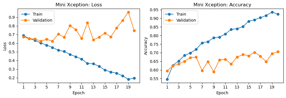
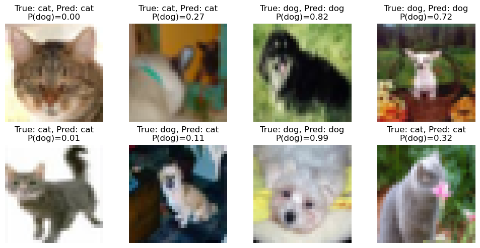
해석·판단: 모델이 구현되었다는 사실과 좋은 분류 성능을 얻었다는 사실은 다르다. 손실과 검증 정확도, 잘못 분류된 이미지를 함께 살펴보자. 채널 분리 합성곱이 파라미터 수를 줄인다고 해서 정확도가 자동으로 높아지는 것은 아니다.
확인 질문: 같은 이미지 분류 문제에서 사전훈련된 Xception과 직접 구현한 Mini Xception의 성능을 비교할 때, 모델 크기뿐 아니라 사전훈련 여부, 훈련 에포크 수, 입력 처리, 검증 데이터 중 무엇을 확인해야 할까?
10.8객체 탐지: 이미지 분류를 넘어
10.8.1객체 탐지: 물체의 종류와 위치를 함께 예측하기
이미지 분류는 이미지 전체의 클래스를 예측한다. 반면 객체 탐지는 이미지 안에 있는 각 객체의 클래스와 위치를 함께 예측한다.
여기서는 모델을 새로 훈련하지 않고, COCO 데이터셋으로 사전훈련된 Faster R-CNN 모델을 사용해 탐지 결과를 살펴본다. 실습의 목적은 높은 성능을 얻는 것이 아니라 탐지 모델의 출력이 무엇을 의미하는지 이해하는 것이다.
import matplotlib.cbook as cbook
from PIL import Image
from torchvision.models.detection import fasterrcnn_resnet50_fpn
from torchvision.models.detection import FasterRCNN_ResNet50_FPN_Weights

sample_path = cbook.get_sample_data('grace_hopper.jpg', asfileobj=False)
detection_image = Image.open(sample_path).convert('RGB')

detection_device = torch.device('cuda' if torch.cuda.is_available() else 'cpu')
weights = FasterRCNN_ResNet50_FPN_Weights.DEFAULT
detector = fasterrcnn_resnet50_fpn(weights=weights).to(detection_device)
detector.eval()

detection_transform = weights.transforms()
coco_categories = weights.meta['categories']

print('Detection device:', detection_device)
print('Sample image size:', detection_image.size)
Downloading: "https://download.pytorch.org/models/fasterrcnn_resnet50_fpn_coco-258fb6c6.pth" to /home/gslee/.cache/torch/hub/checkpoints/fasterrcnn_resnet50_fpn_coco-258fb6c6.pth
100%|██████████| 160M/160M [00:19<00:00, 8.71MB/s]
Detection device: cuda
Sample image size: (512, 600)
10.8.2경계 상자와 신뢰도 확인
객체 탐지 모델은 보통 다음 세 가지를 함께 출력한다.
boxes: 경계 상자 좌표(x1, y1, x2, y2)labels: 예측된 클래스 인덱스scores: 각 예측의 신뢰도
실습에서는 신뢰도(score)가 일정 기준 이상인 예측만 화면에 표시한다.
def run_detection(image, score_threshold=0.70):
    x = detection_transform(image).unsqueeze(0).to(detection_device)
    with torch.no_grad():
        output = detector(x)[0]

    boxes = output['boxes'].detach().cpu().numpy()
    labels = output['labels'].detach().cpu().numpy()
    scores = output['scores'].detach().cpu().numpy()
    keep = scores >= score_threshold
    return boxes[keep], labels[keep], scores[keep]


def show_detection(ax, image, boxes, labels, scores, title):
    ax.imshow(image)
    ax.set_title(title)
    ax.axis('off')
    for box, label, score in zip(boxes, labels, scores):
        x1, y1, x2, y2 = box
        rect = plt.Rectangle((x1, y1), x2 - x1, y2 - y1,
                             fill=False, edgecolor='yellow', linewidth=2)
        ax.add_patch(rect)
        ax.text(x1, max(y1 - 5, 5),
                f"{coco_categories[label]} {score:.2f}",
                color='black', fontsize=9,
                bbox=dict(facecolor='yellow', alpha=0.8, edgecolor='none'))

boxes_07, labels_07, scores_07 = run_detection(detection_image, score_threshold=0.70)

fig, ax = plt.subplots(figsize=(6, 6))
show_detection(ax, detection_image, boxes_07, labels_07, scores_07,
               'Object detection (threshold = 0.70)')
plt.tight_layout()

for label, score in zip(labels_07, scores_07):
    print(f"{coco_categories[label]:>12s}: {score:.3f}")
person: 0.999
tie: 0.955
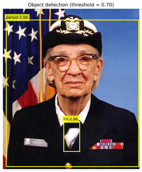
관찰: 이미지 분류였다면 person처럼 이미지 전체에 대한 하나의 클래스를 출력하면 된다. 하지만 객체 탐지에서는 어디에 사람이 있는지를 나타내는 경계 상자도 함께 필요하다.
같은 이미지라도 신뢰도 임곗값을 어떻게 정하느냐에 따라 화면에 남는 예측이 달라질 수 있다.
10.8.3신뢰도 임곗값을 바꾸면 무엇이 달라질까?
임곗값을 낮추면 더 많은 후보를 남기고, 높이면 더 확실한 예측만 남긴다. 이 값은 **오탐(false positive)**과 미탐(false negative) 사이의 균형과 연결된다.
boxes_03, labels_03, scores_03 = run_detection(detection_image, score_threshold=0.30)
boxes_08, labels_08, scores_08 = run_detection(detection_image, score_threshold=0.80)

fig, axes = plt.subplots(1, 2, figsize=(12, 6))
show_detection(axes[0], detection_image, boxes_03, labels_03, scores_03,
               'Threshold = 0.30')
show_detection(axes[1], detection_image, boxes_08, labels_08, scores_08,
               'Threshold = 0.80')
plt.tight_layout()

print('Number of detections at 0.30:', len(scores_03))
print('Number of detections at 0.80:', len(scores_08))
Number of detections at 0.30: 7
Number of detections at 0.80: 2
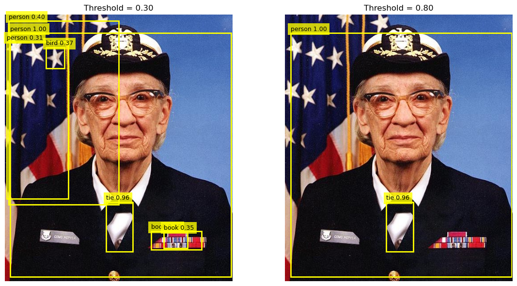
왜 객체 탐지가 컴퓨터 비전의 중요한 응용일까?
자율주행에서는 보행자, 자동차, 신호등의 위치가 필요하다.
의료 영상에서는 병변이 어디에 있는지를 표시해야 한다.
보안 영상에서는 사람이나 물체의 존재와 위치를 함께 확인해야 한다.
즉 객체 탐지는 **무엇이 있는가?**뿐 아니라 **어디에 있는가?**까지 답하려는 문제다.
10.9실습 정리
CNN: 이미지의 공간 구조를 보존하여 국소 필터를 여러 위치에 적용한다.
합성곱: 필터 가중치를 학습하고 출력 특성맵을 만든다.
풀링: 공간 크기를 줄이지만 학습할 파라미터는 없다.
데이터 증식: 훈련 이미지를 다양하게 변형하되 라벨의 의미를 유지한다.
전이 학습: 사전훈련 기저를 재활용한다. 미세 조정은 일부 층을 작은 학습률로 추가 훈련한다.
컴퓨터 비전: 분류·탐지·분할은 예측해야 할 타깃의 형태부터 다르다.
CNN 아키텍처: 잔차 연결, 배치 정규화, 채널 분리 합성곱에는 각각 다른 설계 목적이 있다. Mini Xception에서는 세 기법을 결합하여 이미지 분류 모델로 직접 사용했다.
10.10확인 문제
MNIST CNN의 입력을
(28, 28, 1)로 사용하는 이유는 무엇인가?합성곱 필터 수를 32에서 64로 늘리면 출력의 어떤 차원이 달라지는가?
맥스 풀링과 합성곱의 파라미터 학습 여부는 어떻게 다른가?
Keras의
Conv2D와 PyTorch의Conv2d입력 텐서 순서 차이는 무엇인가?CIFAR-10 고양이·개 분류에서 데이터 증식 결과를 테스트 데이터에 적용하지 않는 이유는 무엇인가?
사전훈련 기저에서
trainable=False를 사용하는 이유는 무엇인가?이미지 분류와 객체 탐지는 타깃의 형태가 어떻게 다른가?
객체 탐지에서 신뢰도 임곗값을 높이면 어떤 변화가 생기는가?
해설 보기
높이·너비 및 흑백 채널 정보를 보존하기 위해서다.
출력 채널 수(마지막 축 또는 PyTorch에서는 두 번째 축)가 달라진다.
합성곱의 필터는 학습하지만, 풀링은 정해진 규칙으로 값을 선택한다.
Keras: NHWC, PyTorch: NCHW다.
평가에서는 훈련 때 사용한 무작위 변환이 아닌 증식하지 않은 검증·테스트 데이터를 사용하여 일반화 성능을 확인하기 위해서다.
사전훈련된 가중치를 유지한 상태에서 새 분류 출력층을 훈련하기 위해서다.
분류는 이미지당 클래스 하나를 예측하고, 객체 탐지는 각 객체의 클래스와 위치를 함께 예측한다.
더 확실한 예측만 남고 탐지 수는 줄어드는 경향이 있다.