2장 신경망의 수학적 구성 요소
감사말: 프랑소와 숄레의 Deep Learning with Python, Second Edition 2장에 사용된 코드에 대한 설명을 담고 있으며 텐서플로우 2.6 버전에서 작성되었습니다. 소스코드를 공개한 저자에게 감사드립니다.
구글 코랩 설정: '런타임 -> 런타임 유형 변경' 메뉴에서 GPU를 지정한다. 이후 아래 명령어를 실행했을 때 오류가 발생하지 않으면 필요할 때 GPU가 자동 사용된다.
!nvidia-smi구글 코랩에서 사용되는 tensorflow 버전을 확인하려면 아래 명령문을 실행한다.
import tensorflow as tf
tf.__version__
tensorflow가 GPU를 사용하는지 여부를 알고 싶으면 주피터 노트북 등 사용하는 편집기 및 파이썬 터미널에서 아래 명령문을 실행한다.
import tensorflow as tf
tf.config.list_physical_devices('GPU')
2.1 신경망 소개
케라스로 MNIST 데이터셋 불러오기
- 손글씨 숫자 인식 용도 데이터셋: 70,000개의 샘플 포함
- 레이블(타깃): 0부터 9까지 10개의 범주(category, class)
- 훈련 세트
- 모델 학습 용도
- 샘플: 28x28 픽셀 크기의 이미지 60,000개
- 테스트 세트
- 학습된 모델 성능 테스트 용도
- 샘플: 28x28 픽셀 크기의 이미지 10,000개
from tensorflow.keras.datasets import mnist
(train_images, train_labels), (test_images, test_labels) = mnist.load_data()
train_images.shape
len(train_labels)
train_labels
test_images.shape
len(test_labels)
test_labels
신경망 구조 지정
아래 신경망의 구조는 다음과 같다.
- 층(layer)
- 2개의 Dense 층 사용
- 입력 데이터로부터 표현(representation) 추출. 즉 입력 데이터를 새로운 표현으로 변환.
- 일종의 데이터 정제를 위한 필터 역할 수행
- 층 연결
Sequential모델 활용- 완전 연결(fully connected). 조밀(densely)하게 연결되었다고 함.
- 첫째 층
- 512개의 유닛(unit) 사용. 즉 512개의 특성값으로 이루어진 표현 추출.
- 활성화 함수(activation function): 렐루(relu) 함수
- 둘째 층
- 10개의 유닛 사용. 10개의 범주를 대상으로 해당 범부에 속할 확률 계산. 모든 확률의 합은 1.
- 활성화 함수: 소프트맥스(softmax) 함수
from tensorflow import keras
from tensorflow.keras import layers
model = keras.Sequential([
    layers.Dense(512, activation="relu"),
    layers.Dense(10, activation="softmax")
])
신경망 컴파일
구조가 지정된 신경망을 훈련이 가능한 모델로 만드는 과정이며 아래 세 가지 사항이 지정되어야 한다.
- 옵티마이저(optimizer): 모델의 성능을 향상시키는 방향으로 가중치를 업데이트하는 알고리즘
- 손실 함수(loss function): 훈련 중 성능 측정 기준
- 모니터링 지표: 훈련과 테스트 과정을 모니터링 할 때 사용되는 평가 지표(metric). 손실 함수값을 사용할 수도 있고 아닐 수도 있음. 아래 코드에서는 정확도(accuracy)만 사용.
model.compile(optimizer="rmsprop",
              loss="sparse_categorical_crossentropy",
              metrics=["accuracy"])
이미지 데이터 전처리
모델이 사용하기 좋은 방식으로 데이터셋의 표현을 0과 1사이의 값으로 구성된
2차원 어레이로 변환한다.
즉, 0부터 255 사이의 정수로 이루어진 (28, 28) 모양의 2차원 어레이로 표현된 이미지를
0부터 1 사이의 부동소수점으로 이루어진 (28*28, ) 모양의 1차원 어레이로 변환한다.
- 훈련 세트 어레이 모양:
(60000, 28*28) - 테스트 세트 어레이 모양:
(10000, 28*28)

그림 출처: 생활코딩: 한 페이지 머신러닝
train_images = train_images.reshape((60000, 28 * 28))
train_images = train_images.astype("float32") / 255   # 0과 1사이의 값
test_images = test_images.reshape((10000, 28 * 28))
test_images = test_images.astype("float32") / 255     # 0과 1사이의 값
모델 훈련
컴파일된 객체 모델을 훈련한다.
fit()메서드 호출: 훈련 세트와 레이블을 인자로 사용epoths: 에포크(전체 훈련 세트 대상 반복 훈련 횟수)batch_size: 가중치 업데이트 한 번 실행할 때 사용되는 샘플 수
model.fit(train_images, train_labels, epochs=5, batch_size=128)
훈련 세트 대상으로 최종 98.98%의 정확도 성능을 보인다.
모델 활용: 예측하기
훈련에 사용되지 않은 손글씨 숫자 이미지 10장에 대한 모델 예측값을 확인하기 위해
predict() 메서드를 이용한다.
test_digits = test_images[0:10]
predictions = model.predict(test_digits)
각 이미지에 대한 예측값은 이미지가 각 범주에 속할 확률을 갖는 길이가 10인 1차원 어레이로 계산된다. 첫째 이미지에 대한 예측값은 다음과 같다.
predictions[0]
가장 높은 확률값을 갖는 인덱스는 7이다.
predictions[0].argmax()
첫째 이미지가 가리키는 숫자가 7일 확률이 99.99%이다.
predictions[0][7]
실제로 첫째 이미지의 레이블이 7임을 확인할 수 있다.
test_labels[0]
테스트 성능
테스트 세트 전체에 대한 성능 평가는 evaluate() 메서드를 활용한다.
성능평가에 사용되는 지표는 앞서 모델을 컴파일할 때 지정한 정확도(accuracy)가 사용된다.
test_loss, test_acc = model.evaluate(test_images, test_labels)
print(f"test_acc: {test_acc}")
테스트 세트에 대한 정확도는 98% 정도이며 훈련 세트에 대한 정확도 보다 낮다. 이는 모델이 훈련 세트에 과대적합(overfitting) 되었음을 의미한다. 과대적합에 대해서는 나중에 보다 자세히 다룰 것이다.
2.2 신경망에 사용되는 데이터 표현
앞서 텐서(tensor)라고 불리는 넘파이 어레이(NumPy array)를 이용하여 데이터를 표현하였다.
텐서는 기본적으로 숫자를 담은 컨테이너(container)이며, 행렬의 경우 2 개의 차원으로 구성된 텐서로 표현된다. 텐서의 차원은 임의로 많을 수 있으며, 텐서에 사용되는 차원을 축(axis)이라 부르기도 한다. 차원의 수를 랭크(rank)라 부른다. 즉 행렬은 랭크가 2인 텐서이다.
주의사항: tensorflow 라이브러리가 제공하는 Tensor 자료형은 NumPy의 어레이
자료형과 매우 비슷하다. 다만 Tensor는 GPU를 활용한 연산을 지원하고
넘파이 어레이는 그렇지 않다.
하지만 두 자료형 사이의 형변환이 존재하여 keras 모델 훈련 등
필요할 때 적절한 형변환이 자동으로 이루어진다.
스칼라(0D 텐서)
숫자 하나로 이루어진 텐서를 스칼라(scalar)라고 하며,
차원이 없다는 의미에서 0D 텐서로 부른다.
넘파이의 경우 float32, float64 등이 스칼라이다.
import numpy as np

x = np.array(12)
x
텐서의 랭크는 ndim 속성이 가리킨다.
x.ndim
벡터 (1D 텐서)
벡터는 1개의 차원(축)을 갖는다. 넘파이의 경우 1차원 어레이가 벡터이다.
x = np.array([12, 3, 6, 14, 7])
x
x.ndim
주의사항: 벡터의 길이를 차원이라 부르기도 하는 점에 주의해야 한다. 예를 들어, 위 벡터는 5D 벡터이다.
행렬(2D 텐서)
행렬은 동일한 크기의 벡터로 이루어진 어레이며, 행(row)과 열(column) 두 개의 축을 갖는다. 넘파이의 2차원 어레이가 2D 텐서이다.
x = np.array([[5, 78, 2, 34, 0],
              [6, 79, 3, 35, 1],
              [7, 80, 4, 36, 2]])
x.ndim
3D 이상의 고차원 텐서
2D 텐서로 이루어진 어레이가 3D 텐서이며, 이 과정을 반복해서 4D 이상의 고차원 텐서도 생성할 수 있다. 딥러닝에서 다루는 텐서는 보통 최대 4D이며, 동영상 데이터를 다룰 때 5D 텐서도 사용한다.
x = np.array([[[5, 78, 2, 34, 0],
               [6, 79, 3, 35, 1],
               [7, 80, 4, 36, 2]],
              [[5, 78, 2, 34, 0],
               [6, 79, 3, 35, 1],
               [7, 80, 4, 36, 2]],
              [[5, 78, 2, 34, 0],
               [6, 79, 3, 35, 1],
               [7, 80, 4, 36, 2]]])
x.ndim
텐서의 주요 속성
- 축의 수(랭크,
ndim)- 텐서에 사용된 축(차원)의 개수
- 음이 아닌 정수
- 모양(
shape)- 각각의 축에 사용된 (벡터의) 차원 수
- 정수로 이루어진 튜플
- 자료형(
dtype)- 텐서에 사용된 항목들의 (통일된) 자료형
float16,float32,float64,int8,string등이 가장 많이 사용됨.- 8, 16, 32, 64 등의 숫자는 해당 숫자를 다루는 데 필요한 메모리의 비트(bit) 크기를 가리킴. 즉, 텐서에 사용되는 항목들을 일괄된 크기의 메모리로 처리함.
MNIST 훈련 세트를 대상으로 언급된 속성을 확인해보자. 앞서 모양을 변형하였기에 다시 원본 데이터를 불러온다.
from tensorflow.keras.datasets import mnist
(train_images, train_labels), (test_images, test_labels) = mnist.load_data()
train_images.ndim
train_images.shape
train_images.dtype
다섯 번째 이미지 확인하기
훈련 세트에 포함된 이미지 중에서 다섯 번째 이미지를 직접 확인해보자.
이를 위해 pyplot 모듈의 imshow() 함수를 이용한다.
import matplotlib.pyplot as plt

digit = train_images[4]
plt.imshow(digit, cmap=plt.cm.binary)
plt.show()

다섯 번째(4번 인덱스) 이미지는 실제로 숫자 9를 가리킨다.
train_labels[4]
넘파이를 이용한 텐서 조작
인덱싱(indexing)
텐서에 포함된 특정 인덱스의 항목 선택하려면 인덱싱을 사용한다.
train_labels[4]
슬라이싱
텐서에 포함된 특정 구간에 포함된 인덱스에 해당하는 항목으로 이루어진 텐서를 생성할 때 슬라이싱을 사용한다.
my_slice = train_images[10:100]
my_slice.shape
:는 지정된 축의 인덱스 전체를 대상으로 한다.
따라서 위 코드는 아래 두 코드와 동일한 기능을 수행한다.
my_slice = train_images[10:100, :, :]
my_slice.shape
my_slice = train_images[10:100, 0:28, 0:28]
my_slice.shape
이미지 전체를 대상으로 오른편 하단의 14x14 픽셀만 추출하려면 다음과 같이
슬라이싱을 진행한다.
my_slice = train_images[:, 14:, 14:]
이미지 전체를 대상으로 중앙에 위치한 14x14 픽셀만 추출하려면 다음과 같이
슬라이싱을 진행한다.
음의 인덱스는 끝(-1번 인덱스)에서부터 역순으로 세어진 인덱스를 가리킨다.
my_slice = train_images[:, 7:-7, 7:-7]
데이터 배치(묶음)
케라스를 포함하여 대부분의 딥러닝 모델은 훈련 세트 전체를 한꺼번에 처리하지 않고
지정된 크기(batch_size)의 배치(batch)로 나주어 처리한다.
앞서 살펴본 모델의 배치 크기는 128이었다.
샘플 축 또는 샘플 차원
딥러닝에 사용되는 모든 훈련 세트의 0번 축(axis 0)은 포함된 샘플 각각을 가리키는 샘플 축(samples axis)이며, 샘플 차원(samples dimension)이라고도 불린다. 특별히 배치 텐서와 관련해서는 0번 축(axis 0)을 배치 축(batch axis) 또는 배치 차원(batch dimension)이라고 부른다.
- 첫째 배치
batch = train_images[:128]
- 둘째 배치
batch = train_images[128:256]
- n 번째 배치
n = 3 # 임의의 n이라고 가정해야 함

batch = train_images[128 * n:128 * (n + 1)]
2.3 텐서 연산
신경망 모델의 훈련은 기본적으로 텐서와 관련된 몇 가지 연산으로 이루어진다. 예를 들어 이전 신경망에 사용된 케라스 레이어를 살펴보자.
keras.layers.Dense(512, activation="relu")
keras.layers.Dense(10, activation="softmax")
위 두 개의 층이 하는 일은 데이터셋의 변환이며 실제로 이루어지는 연산은 다음과 같다.
1층
output1 = relu(dot(input1, W1) + b1)
2층
output2 = softmax(dot(input2, W2) + b2)
점곱(
dot(input, W)): 입력 텐서와 가중치 텐서의 곱- 덧셈(
dot(input, W) + b): 점곱의 결과 텐서와 벡터b의 합 relu함수:relu(x) = max(x, 0)softmax함수: 10개 범주 각각에 속할 확률 계산

그림 출처: 생활코딩: 한 페이지 머신러닝
항목별 연산
넘파이의 어레이 연산처럼 텐서의 연산도 항목별로 이루어진다.
예를 들어, relu() 함수도 각 항목에 적용되며,
실제로 아래와 같이 구현할 수 있다.
def naive_relu(x):
    assert len(x.shape) == 2
    x = x.copy()
    for i in range(x.shape[0]):
        for j in range(x.shape[1]):
            x[i, j] = max(x[i, j], 0)
    return x
덧셈도 동일하다.
def naive_add(x, y):
    assert len(x.shape) == 2
    assert x.shape == y.shape
    x = x.copy()
    for i in range(x.shape[0]):
        for j in range(x.shape[1]):
            x[i, j] += y[i, j]
    return x
넘파이의 경우 항목별 연산을 병렬처리가 가능하며 매우 효율적으로 작동하는 저수준 언어로 구현되어 있다. 아래 두 코드는 넘파이를 활용할 때와 그렇지 않을 때의 처리속도의 차이를 잘 보여준다.
import time

x = np.random.random((20, 100))
y = np.random.random((20, 100))

t0 = time.time()
for _ in range(1000):
    z = x + y
    z = np.maximum(z, 0.)
print(f"Took: {time.time() - t0:.2f}초")
t0 = time.time()
for _ in range(1000):
    z = naive_add(x, y)
    z = naive_relu(z)
print(f"Took: {time.time() - t0:.2f}초")
텐서플로우 또한 GPU로 병렬 처리를 효율적으로 수행하는 항목변 연산을 지원한다.
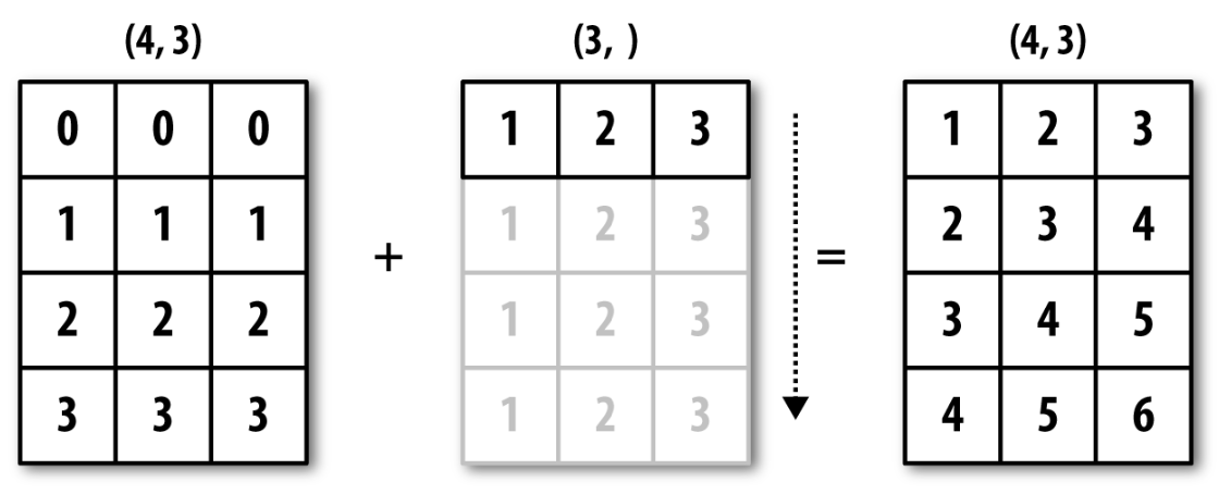
브로드캐스팅(Broadcasting)
아래 식은 2D 텐서와 벡터(1D 텐서)의 합을 계산한다.
dot(input, W) + b
차원이 다른 텐서의 합과 차를 계산하려면 모양을 먼저 맞춰주어야 한다.
위 표현식의 계산과정에서 b를 먼저 dot(input, W)의 모양과 일치하도록
브로드캐스팅 한다.
아래 코드는 2D 텐서와 1D 텐서의 합이 이루어지는 과정을 보여준다.
import numpy as np
X = np.random.random((32, 10))
y = np.random.random((10,))
y
y텐서 2D로 변환:(10,)모양의 1D 텐서를(1, 10)모양의 2D 텐서로 변환
y2 = np.expand_dims(y, axis=0)
y2
(32, 10)모양의 2D 텐서로 변환: 0번 행을 32번 복사해서 추가
Y = np.concatenate([y2] * 32, axis=0)
Y.shape
((X + y) == (X + Y)).all()
이어지는 코드는 아래 형식의 브로드캐스팅을 직접 구현한다.
def naive_add_matrix_and_vector(x, y):
    assert len(x.shape) == 2
    assert len(y.shape) == 1
    assert x.shape[1] == y.shape[0]
    x = x.copy()
    for i in range(x.shape[0]):
        for j in range(x.shape[1]):
            x[i, j] += y[j]
    return x
아래 코드는 차원이 다른 두 텐서에 대해 항목별 최댓값을 계산하는 것이 브로드캐스팅 덕분에 가능함을 보여준다.
import numpy as np
x = np.random.random((64, 3, 32, 10))
y = np.random.random((32, 10))
z = np.maximum(x, y)
텐서 점곱
텐서의 점곱(dot product)은 차원에 따라 다른 계산을 수행한다.
- 두 벡터의 점곱
x = np.random.random((32,))
y = np.random.random((32,))
z = np.dot(x, y)
z
직접 구현하면 다음과 같다.
def naive_vector_dot(x, y):
    assert len(x.shape) == 1
    assert len(y.shape) == 1
    assert x.shape[0] == y.shape[0]
    z = 0.
    for i in range(x.shape[0]):
        z += x[i] * y[i]
    return z
naive_vector_dot(x, y)
- 2D 텐서와 벡터의 점곱 (방식 1)
x = np.random.random((2,3))
y = np.random.random((3,))
z = np.dot(x, y)
z
def naive_matrix_vector_dot(x, y):
    assert len(x.shape) == 2
    assert len(y.shape) == 1
    assert x.shape[1] == y.shape[0]
    z = np.zeros(x.shape[0])
    for i in range(x.shape[0]):
        for j in range(x.shape[1]):
            z[i] += x[i, j] * y[j]
    return z
naive_matrix_vector_dot(x, y)
- 2D 텐서와 벡터의 점곱 (방식 2)
def naive_matrix_vector_dot(x, y):
    z = np.zeros(x.shape[0])
    for i in range(x.shape[0]):
        z[i] = naive_vector_dot(x[i, :], y)
    return z
naive_matrix_vector_dot(x, y)
- 2D 텐서와 2D 텐서의 점곱 (행렬의 곱)
x = np.random.random((2,3))
y = np.random.random((3,4))
z = np.dot(x, y)
z
def naive_matrix_dot(x, y):
    assert len(x.shape) == 2
    assert len(y.shape) == 2
    assert x.shape[1] == y.shape[0]
    z = np.zeros((x.shape[0], y.shape[1]))
    for i in range(x.shape[0]):
        for j in range(y.shape[1]):
            row_x = x[i, :]
            column_y = y[:, j]
            z[i, j] = naive_vector_dot(row_x, column_y)
    return z
naive_matrix_dot(x, y)
텐서 모양 변환
앞서 아래 코드에서 텐서의 모양을 변환했다.
train_images = train_images.reshape((60000, 28 * 28))
즉, MNIST 훈련 세트가 원래 (60000, 28, 28) 모양의 3D 텐서로 주어졌는데
신경망 모델의 입력값으로 사용하기 위해 (60000, 28 * 28) 모양의 2D 텐서로 변환하는
전처리 과정을 사용했다.
train_images = train_images.reshape((60000, 28 * 28))
텐서의 모양 변환은 지정된 모양의 텐서를 생성하기 위해 기존 텐서의 행(row)과 열(column)을 새롭게 정렬한다. 따라서 항목의 개수는 변하지 않는다. 아래 코드는 텐서의 모양 변환을 설명하는 간단한 예제를 보여준다.
x = np.array([[0., 1.],
             [2., 3.],
             [4., 5.]])
x.shape
x = x.reshape((6, 1))
x
행렬의 전치
행렬(2D 텐서)의 행과 열을 바꾸는 전치(transposition) 또한 행렬의 모양 변환이다.
x = np.zeros((300, 20))
x = np.transpose(x)
x.shape
2.4 신경망의 엔진: 그레이디언트 기반 최적화
텐서플로우의 그레이디언트 테이프
- 미분 자동화: 역전파에 필요한 그레이디언트 자동 계산
- 그레이디언트 테이프(gradient tape): 임의의 텐서 연산에 대해 지정된 변수에 대한 그레이디언트를 미리 계산해 놓는 독립적인 장치
tf.Variable객체: 그레이디언트 테이프를 사용하려면 변수를tf.Variable클래스의 인스턴스로 선언해야 함.
하나의 변수에 대한 그레이디언트
import tensorflow as tf

x = tf.Variable(0.)

with tf.GradientTape() as tape:
    y = x**2 + 2*x + 3

grad_of_y_wrt_x = tape.gradient(y, x)
grad_of_y_wrt_x
임의의 텐서 연산에 대한 그레이디언트
x = tf.Variable(tf.random.uniform((2, 2)))

with tf.GradientTape() as tape:
    y = x**2 + 3

grad_of_y_wrt_x = tape.gradient(y, x)
변수 x의 모양은 다음과 같다.
y를 x의 함수로 표현하면 다음과 같다.
텐서 x에 대한 그레이디언트는 다음과 같다.
grad_of_y_wrt_x
x
변수들의 리스트에 대한 그레이언트
W = tf.Variable(tf.random.uniform((2, 2)))
b = tf.Variable(tf.zeros((2,)))
x = tf.random.uniform((2, 2))

with tf.GradientTape() as tape:
    y = tf.matmul(x, W) + b

grad_of_y_wrt_W_and_b = tape.gradient(y, [W, b])
텐서 x와 변수 W, b의 모양은 다음과 같다.
y를 W와 b의 함수로 표현하면 다음과 같다.
텐서 x에 대한 그레이디언트는 다음과 같다.
grad_of_y_wrt_W_and_b
x
2.5 신경망 구현: 밑바닥부터
케라스가 아닌 순수 텐서플로우 API 만을 이용해서 앞서 사용한 MINST 분류 신경망 모델에 사용된 클래스를 직접 구현한다.
MNIST 케라스 모델
앞서 사용한 케라스 모델과 훈련 과정은 다음과 같다.
- MNIST 데이터 불러오기와 모양 및 형 변환
(train_images, train_labels), (test_images, test_labels) = mnist.load_data()
train_images = train_images.reshape((60000, 28 * 28))
train_images = train_images.astype("float32") / 255
test_images = test_images.reshape((10000, 28 * 28))
test_images = test_images.astype("float32") / 255
- 케라스 모델 선언
model = keras.Sequential([
    layers.Dense(512, activation="relu"),
    layers.Dense(10, activation="softmax")
])
- 케라스 모델 컴파일
model.compile(optimizer="rmsprop",
              loss="sparse_categorical_crossentropy",
              metrics=["accuracy"])
- 케라스 모델 훈련
model.fit(train_images, train_labels, epochs=5, batch_size=128)
텐서플로우만을 사용한 MNIST 모델 구현
단순한 Dense 클래스
- 입력 크기(
input_size)와 출력 크기(output_size) 함께 지정. __call__()메서드: 클래스를 함수처럼 호출할 때 사용되는 매직 메서드@property: 메서드를 속성 변수처럼 작동하도록 하는 데코레이터weights: 가중치 텐서들의 리스트
import tensorflow as tf

class NaiveDense:
    def __init__(self, input_size, output_size, activation):
        self.activation = activation

        # 가중치 행렬 선언 및 초기화
        w_shape = (input_size, output_size)
        w_initial_value = tf.random.uniform(w_shape, minval=0, maxval=1e-1)
        self.W = tf.Variable(w_initial_value)    # 가중치를 tf.Variable로 선언

        b_shape = (output_size,)
        b_initial_value = tf.zeros(b_shape)
        self.b = tf.Variable(b_initial_value)    # 편향을 tf.Variable로 선언

    def __call__(self, inputs):
        return self.activation(tf.matmul(inputs, self.W) + self.b)

    @property
    def weights(self):
        return [self.W, self.b]
단순한 Sequential 클래스
__call__()메서드: 포함된 층의__call_()메서드 연속 적용weights: 포함된 모든 층의 가중치 텐서를 항목으로 갖는 리스트
class NaiveSequential:
    def __init__(self, layers):
        self.layers = layers

    def __call__(self, inputs):
        x = inputs
        for layer in self.layers:
            x = layer(x)
        return x

    @property
    def weights(self):
        weights = []
        for layer in self.layers:
            weights += layer.weights
        return weights
MNIST 훈련 모델 선언
model = NaiveSequential([
    NaiveDense(input_size=28 * 28, output_size=512, activation=tf.nn.relu),
    NaiveDense(input_size=512, output_size=10, activation=tf.nn.softmax)
])
weights 리스트의 길이가 4로 확인된다.
이유는 각 층에서 두 개씩 추가되었기 때문이다.
assert len(model.weights) == 4
배치(묶음) 생성 클래스
지정된 크기의 배치를 차례대로 생성하는 클래스이며, 일종의 제너레이터(generator) 역할을 수행한다.
import math

class BatchGenerator:
    def __init__(self, images, labels, batch_size=128):
        assert len(images) == len(labels)
        self.index = 0
        self.images = images
        self.labels = labels
        self.batch_size = batch_size
        self.num_batches = math.ceil(len(images) / batch_size)    # 배치 개수

    # 다음 배치 생성 메서드
    def next(self):
        images = self.images[self.index : self.index + self.batch_size]
        labels = self.labels[self.index : self.index + self.batch_size]
        self.index += self.batch_size
        return images, labels
훈련 단계
하나의 데이터 배치를 학습한 후에 가중치를 업데이트하는 기능을 수행하는 함수를 정의한다.
def one_training_step(model, images_batch, labels_batch):
    # 그레이디언트 테이프 활용
    with tf.GradientTape() as tape:
        predictions = model(images_batch)
        per_sample_losses = tf.keras.losses.sparse_categorical_crossentropy(
            labels_batch, predictions)
        average_loss = tf.reduce_mean(per_sample_losses)

    # 그레이디언트 계산
    gradients = tape.gradient(average_loss, model.weights)
    # 가중치 업데이트
    update_weights(gradients, model.weights)   # 가중치 업데이트 함수

    return average_loss
가중치 업데이트 함수는 다음과 같다.
assign_sub()메서드:tf.Variable()자료형의 메서드. 항목별 뺄셈 실행.
learning_rate = 1e-3

def update_weights(gradients, weights):
    for g, w in zip(gradients, model.weights):
        w.assign_sub(g * learning_rate)
주의사항: 가중치 업데이트 함수를 직접 구현하는 일은 매우 드물 것이다.
대신에 케라스의 Optimizer 인스턴스를 사용할 것을 권장한다.
예를 들어 아래 코드는 SGD 옵티마이저를 사용한다.
from tensorflow.keras import optimizers

optimizer = optimizers.SGD(learning_rate=1e-3)

def update_weights(gradients, weights):
    optimizer.apply_gradients(zip(gradients, weights))
훈련 반복: 모델 학습
fit() 메서드의 역할을 수행하는 함수는 다음과 같다.
def fit(model, images, labels, epochs, batch_size=128):
    for epoch_counter in range(epochs):
        print(f"Epoch {epoch_counter}")
        batch_generator = BatchGenerator(images, labels)
        for batch_counter in range(batch_generator.num_batches):
            images_batch, labels_batch = batch_generator.next()
            loss = one_training_step(model, images_batch, labels_batch)

            # 100개의 배치를 검사할 때 마다 손실값 출력
            if batch_counter % 100 == 0:
                print(f"loss at batch {batch_counter}: {loss:.2f}")
MNIST 데이터셋 훈련
from tensorflow.keras.datasets import mnist
(train_images, train_labels), (test_images, test_labels) = mnist.load_data()

train_images = train_images.reshape((60000, 28 * 28))
train_images = train_images.astype("float32") / 255
test_images = test_images.reshape((10000, 28 * 28))
test_images = test_images.astype("float32") / 255

fit(model, train_images, train_labels, epochs=10, batch_size=128)
모델 평가
테스트 세트에 대해 81% 정도의 정확도 성능을 보여준다.
predictions = model(test_images)    # 텐서플로우 자료형
predictions = predictions.numpy()
predicted_labels = np.argmax(predictions, axis=1)
matches = predicted_labels == test_labels
print(f"accuracy: {matches.mean():.2f}")