기본 설정
import numpy as np맷플롯립Matplotlib은 간단한 그래프 도구를 제공하는 라이브러리다.
맷플롯립의 대부분의 함수는 파이플롯pyplot 모듈에 포함되어 있으며
관행적으로 plt 별칭으로 불러온다.
import matplotlib.pyplot as plt24.1분류 대 군집화
분류
각 데이터에 대해 하나의 레이블을 할당한다. 붓꽃의 꽃잎 길이와 너비를 특성으로 사용해서 품종을 레이블로 사용한 결과를 그래프로 그려보자.
먼저 붓꽃 데이터 불러온다.
from sklearn.datasets import load_iris

iris = load_iris() # load_iris(as_frane=False)
X = iris.data
y = iris.targettype(iris)sklearn.utils.BunchX, y 의 자료형은 넘파이 어레이다.
type(X)numpy.ndarrayX[:5]array([[5.1, 3.5, 1.4, 0.2],
[4.9, 3. , 1.4, 0.2],
[4.7, 3.2, 1.3, 0.2],
[4.6, 3.1, 1.5, 0.2],
[5. , 3.6, 1.4, 0.2]])type(y)numpy.ndarrayy[:5]array([0, 0, 0, 0, 0])품종 종류는 다음과 같다.
iris.target_namesarray(['setosa', 'versicolor', 'virginica'], dtype='<U10')품종별 다른 색상으로 산점도를 그리기 위해 부울 인덱싱과 인덱싱을 함께 사용한다.
plt.plot(X[y==0, 2], X[y==0, 3], "yo", label="Iris setosa")
plt.plot(X[y==1, 2], X[y==1, 3], "bs", label="Iris versicolor")
plt.plot(X[y==2, 2], X[y==2, 3], "g^", label="Iris virginica")

plt.xlabel("Petal length")
plt.ylabel("Petal width")
plt.legend()
plt.grid()

plt.show()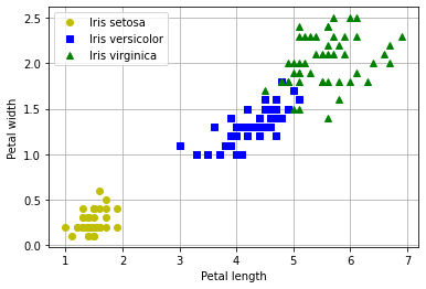
군집화
군집cluster은 유사한 대상들의 모음을 가리킨다. 예를 들어, 산이나 공원에서 볼 수 있는 이름은 모르지만 동일 품종의 꽃으로 이루어진 군집 등을 생각하면 된다. 군집화clustering는 대상들을 나누어 군집을 형성하는 것을 말한다.
각 샘플에 하나의 그룹을 할당한다는 점에서 분류와 유사하다. 하지만 각 샘플에 대해 레이블을 할당하는 게 아니라 유사한 샘플들의 군집으로 구분한다는 점에서 다르다.
아래 그림은 아이리스 붓꽃 데이터에 대한 군집화의 결과를 보여준다. 분류는 세 개의 품종을 매우 잘 분류하지만 군집은 세토사 군집과 나머지 군집으로 구분할 뿐이다.
plt.scatter(X[y==0, 2], X[y==0, 3], c="k", marker=".")
plt.scatter(X[(y==1) | (y==2), 2], X[(y==1) | (y==2), 3], c="b", marker=".")

plt.xlabel("Petal length")
plt.ylabel("Petal width")
plt.grid()

plt.show()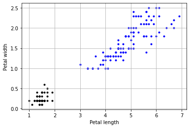
24.2서브플롯 활용
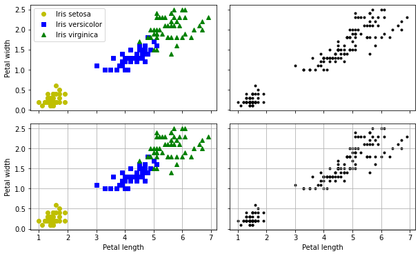
분류와 군집 그래프 여러 개를 동시에 그리기 위해 서브플롯을 활용하는 세 가지 방식을 소개한다.
방식 1: Figure 객체의 add_subplot() 메서드 활용
add_subplot() 함수의 반환값은 Axes 객체다.
Axes 객체는 그래프와 관련된 많은 기능을 지원한다.
plt.rc('figure', figsize=(10, 6))

fig = plt.figure()

ax1 = fig.add_subplot(2, 2, 1)
ax2 = fig.add_subplot(2, 2, 2)
ax3 = fig.add_subplot(2, 2, 3)
ax4 = fig.add_subplot(2, 2, 4)

ax1.plot(X[y==0, 2], X[y==0, 3], "yo", label="Iris setosa")
ax1.plot(X[y==1, 2], X[y==1, 3], "bs", label="Iris versicolor")
ax1.plot(X[y==2, 2], X[y==2, 3], "g^", label="Iris virginica")
ax1.set_ylabel("Petal width")
ax1.tick_params(labelbottom=False)
ax1.legend()

ax2.scatter(X[y==0, 2], X[y==0, 3], c="k", marker=".")
ax2.scatter(X[(y==1) | (y==2), 2], X[(y==1) | (y==2), 3], c="b", marker=".")
ax2.tick_params(labelleft=False, labelbottom=False)

ax3.plot(X[y==0, 2], X[y==0, 3], "yo", label="Iris setosa")
ax3.plot(X[y==1, 2], X[y==1, 3], "bs", label="Iris versicolor")
ax3.plot(X[y==2, 2], X[y==2, 3], "g^", label="Iris virginica")
ax3.set_xlabel("Petal length")
ax3.set_ylabel("Petal width")
ax3.grid()

ax4.scatter(X[y==0, 2], X[y==0, 3], c="k", marker=".")
ax4.scatter(X[(y==1) | (y==2), 2], X[(y==1) | (y==2), 3], c="b", marker=".")
ax4.set_xlabel("Petal length")
ax4.tick_params(labelleft=False)
ax4.grid()

fig.subplots_adjust(wspace=0.07, hspace=0.12) # 상하좌우 여백
# plt.subplots_adjust(wspace=0.07, hspace=0.12) # 상하좌우 여백

plt.show()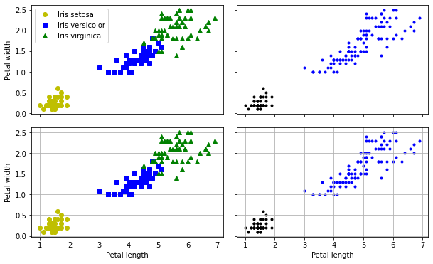
방식 2: plt.subplots() 함수와 Axes 객체 활용
plt.subplots() 함수의 반환값은 Figure 객체와 Axes 객체의 어레이로 구성된 튜플이다.
plt.rc('figure', figsize=(10, 6))

fig, axes = plt.subplots(2, 2, sharex=True, sharey=True)

axes[0, 0].plot(X[y==0, 2], X[y==0, 3], "yo", label="Iris setosa")
axes[0, 0].plot(X[y==1, 2], X[y==1, 3], "bs", label="Iris versicolor")
axes[0, 0].plot(X[y==2, 2], X[y==2, 3], "g^", label="Iris virginica")
axes[0, 0].set_ylabel("Petal width")
axes[0, 0].legend()

axes[0, 1].scatter(X[y==0, 2], X[y==0, 3], c="k", marker=".")
axes[0, 1].scatter(X[(y==1) | (y==2), 2], X[(y==1) | (y==2), 3], c="b", marker=".")

axes[1, 0].plot(X[y==0, 2], X[y==0, 3], "yo", label="Iris setosa")
axes[1, 0].plot(X[y==1, 2], X[y==1, 3], "bs", label="Iris versicolor")
axes[1, 0].plot(X[y==2, 2], X[y==2, 3], "g^", label="Iris virginica")
axes[1, 0].set_xlabel("Petal length")
axes[1, 0].set_ylabel("Petal width")
axes[1, 0].grid()

axes[1, 1].scatter(X[y==0, 2], X[y==0, 3], c="k", marker=".")
axes[1, 1].scatter(X[(y==1) | (y==2), 2], X[(y==1) | (y==2), 3], c="b", marker=".")
axes[1, 1].set_xlabel("Petal length")
axes[1, 1].grid()

fig.subplots_adjust(wspace=0.07, hspace=0.12) # 상하좌우 여백
# plt.subplots_adjust(wspace=0.07, hspace=0.12) # 상하좌우 여백

plt.show()
방식 3: plt.subplot() 함수와 Axes 객체 활용
plt.subplot() 함수는 Figure 객체에 Axes 객체를 하나 추가한다.
해당 Axes 객체에 대한 설정은 바로 실행해야 한다.
plt.figure(figsize=(10, 6))

plt.subplot(221)
plt.plot(X[y==0, 2], X[y==0, 3], "yo", label="Iris setosa")
plt.plot(X[y==1, 2], X[y==1, 3], "bs", label="Iris versicolor")
plt.plot(X[y==2, 2], X[y==2, 3], "g^", label="Iris virginica")
plt.ylabel("Petal width")
plt.tick_params(labelbottom=False)
plt.legend()

plt.subplot(222)
plt.scatter(X[y==0, 2], X[y==0, 3], c="k", marker=".")
plt.scatter(X[(y==1) | (y==2), 2], X[(y==1) | (y==2), 3], c="b", marker=".")
plt.tick_params(labelleft=False, labelbottom=False)

plt.subplot(223)
plt.plot(X[y==0, 2], X[y==0, 3], "yo", label="Iris setosa")
plt.plot(X[y==1, 2], X[y==1, 3], "bs", label="Iris versicolor")
plt.plot(X[y==2, 2], X[y==2, 3], "g^", label="Iris virginica")
plt.xlabel("Petal length")
plt.ylabel("Petal width")
plt.grid()

plt.subplot(224)
plt.scatter(X[y==0, 2], X[y==0, 3], c="k", marker=".")
plt.scatter(X[(y==1) | (y==2), 2], X[(y==1) | (y==2), 3], c="b", marker=".")
plt.xlabel("Petal length")
plt.tick_params(labelleft=False)
plt.grid()

plt.subplots_adjust(wspace=0.07, hspace=0.12) # 상하좌우 여백

plt.show()
다음과 같이 Axes 객체를 변수에 할당하고 활용할 수도 있다.
plt.figure(figsize=(10, 6))

ax1 = plt.subplot(221)
ax1.plot(X[y==0, 2], X[y==0, 3], "yo", label="Iris setosa")
ax1.plot(X[y==1, 2], X[y==1, 3], "bs", label="Iris versicolor")
ax1.plot(X[y==2, 2], X[y==2, 3], "g^", label="Iris virginica")
ax1.set_ylabel("Petal width")
ax1.tick_params(labelbottom=False)
ax1.legend()

ax2 = plt.subplot(222)
ax2.scatter(X[:, 2], X[:, 3], c="k", marker=".")
ax2.tick_params(labelleft=False, labelbottom=False)

ax3 = plt.subplot(223)
ax3.plot(X[y==0, 2], X[y==0, 3], "yo", label="Iris setosa")
ax3.plot(X[y==1, 2], X[y==1, 3], "bs", label="Iris versicolor")
ax3.plot(X[y==2, 2], X[y==2, 3], "g^", label="Iris virginica")
ax3.set_xlabel("Petal length")
ax3.set_ylabel("Petal width")
ax3.grid()

ax4 = plt.subplot(224)
ax4.scatter(X[:, 2], X[:, 3], c="k", marker=".")
ax4.set_xlabel("Petal length")
ax4.tick_params(labelleft=False)
ax4.grid()

plt.subplots_adjust(wspace=0.07, hspace=0.12) # 상하좌우 여백

plt.show()